Introduction
On this page we give a concise introductory overview of some of the main topics involving autonomous flight and vehicle autonomy in general. They are grouped into four chapters:
- Path Planning
- Vehicle Control
- Vehicle State Estimation (position, velocity, attitude, etc., from onboard sensors)
- Computer Vision
Many of the examples below, especially the visual presentations of the simulations, originate from Udacity’s Flying Car and Autonomous Flight Engineer Nanodegree and the Self-Driving Car Engineer Nanodegree programs. We encourage you to take a look at these programs on the Udacity website.
We currently offer short courses in vehicle state estimation and vehicle control, which are somewhat complementary in nature. They dive deeper into selected topics than, for instance, the above Nanodegrees, but without the spectacular visuals and without offering the broad overview of vehicle autonomy that the above programs provide. They are also much heavier on the mathematics, including derivations and not just application of formulas. They are suitable either for people who have a need for only a single topic in more detail (e.g. attitude estimation from iPhone IMU data), or who have taken courses similar to the above and want to improve their understanding of certain aspects.
The prerequisites for all our autonomous flight courses are a solid familiarity with Python (including classes), and basic familiarity with undergraduate-level linear algebra (vector spaces, matrices, matrix inversion, etc.) and multivariable calculus (total and partial derivatives, integrals, etc.). If you lack some of these prerequisites, we can help you obtain them. There are also plenty of introductory math and programming courses available on online learning platforms like Coursera, many of which you can audit for free.
Path Planning
Path Planning with A* and Bresenham Algorithms
Before we can start a flight, we need to ask the three basic questions of navigation: Where am I? Where am I going? How am I going to get there? If we have a map and know the starting and end points of our journey, the first two questions are trivially answered. The third one is more involved, as we need to avoid obstacles.
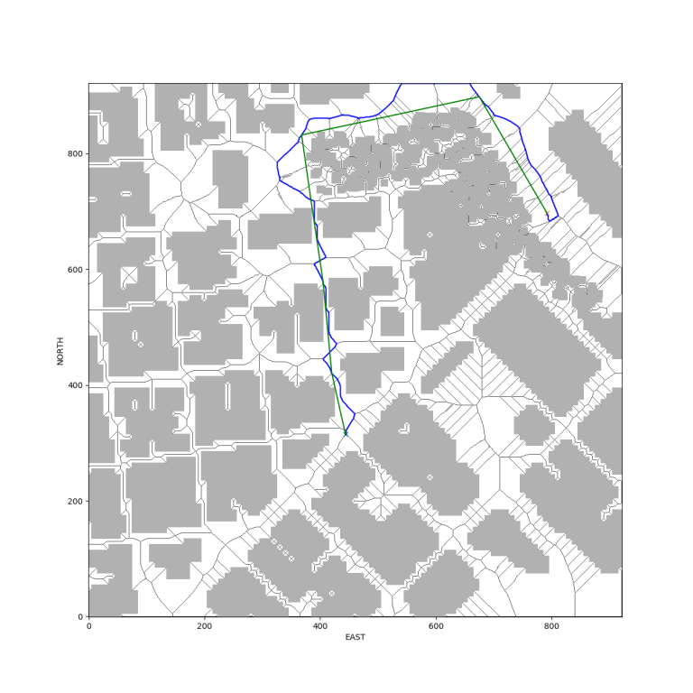
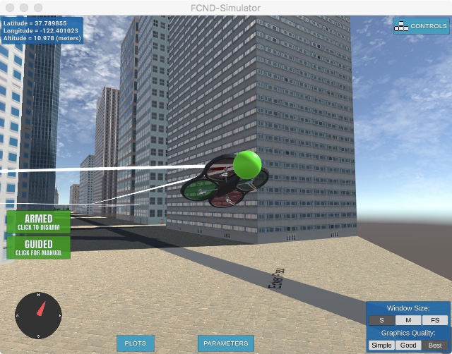
In the image on the top right we show a planned path for a drone flight in downtown San Francisco. First we constructed a medial axis skeleton between all the obstacles. Then we found a path (blue) along the medial axis skeleton using the A* algorithm. Finally, a modified Bresenham algorithm was used to streamline the flight path by removing superfluous waypoints on segments with no obstacles in between (shown in green). The bottom image illustrates a drone following the path and turning at a waypoint (depicted green ball) in Udacity’s FCND simulator. (Click on images for magnified view.)
Adaptive Path Corrections
Path planning must by dynamically adaptive during travel, because unexpected events can occur en route. For instance, another vehicle may get in the way, and the path must be changed temporarily to avoid this unforeseen obstacle. In the video on the right we let a car drive on a freeway in Udacity’s self-driving car simulator and have programed it to avoid other cars by changing lanes. At the same time, excessive accelerations and jerks due to steering motions and braking are to be avoided. The green line indicates the current local path the vehicle is expecting to follow in the near future.
Vehicle Control
3-Axis PID Controller
Vehicle control is achieved with a 3-axis proportional-integral-derivative (PID) controller. It issues commands to the controls of the vehicle based on deviations from the desired position and velocity on the flight path, which enable the vehicle to follow the path which we planned in the above chapter.
For the video on the right, we wrote a PID controller in C++ to fly two quadrotors on a figure-eight flight path in Udacity’s drone simulator. The colored dot denotes the desired location of the drone at any given time. The red drone in he back has an intentional mass misestimate, which an integral term takes care of, resulting in some lag.
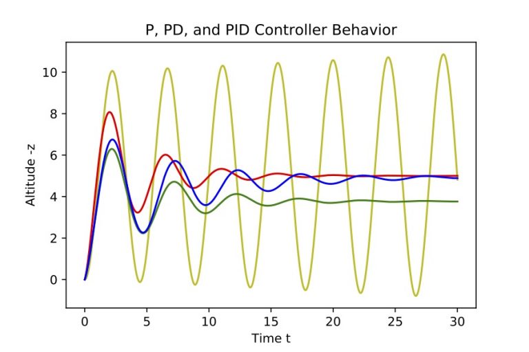
The image on the bottom right illustrates the general properties of a PID controller and the effects of its individual P, I, D components in 1D for a vehicle trying to reach an altitude of 5 meters.
Further Improvement Outlook
On a curved path, we can use a feedforward term to give the vehicle a hint of what will happen next. But the vehicle still does not understand its own kinematics and therefore anything about the future. Proper magnitude of control inputs to path deviations is achieved merely by tuning the gain parameters of the PID controller to reasonable values. This has its limits and can be greatly improved by providing the vehicle with an understanding of a motion model and using model predictive control (MPC), see next section.
Also note that at this point we have still idealistically assumed that the current state of the vehicle is exactly known. We shall relax this assumption in the next chapter on vehicle state estimation further below.
Model Predictive Control (MPC)
Model predictive control (MPC) tries to find the best control input values at a given time to steer the vehicle on a desired track. To this end, the MPC code simulates various sequences of different control inputs, using a vehicle motion model and starting at the current vehicle position (plus any incorporated latency), and the resulting predicted track is compared to the desired track. The best control input sequence is found by assigning a penalty (cost) for track and speed deviations (as well as for control inputs to avoid unnecessary ones), and by minimizing this cost function. Once the best control sequence is found, the car then executes the first of the control inputs of this sequence. The optimization process is then repeated, starting from the current new vehicle state, which never quite matches the predicted one.
Vehicle State Estimation
Kalman Filters and Sensor Fusion
The state of a vehicle can be described by a 12-dimensional state vector consisting of position, velocity, Euler angles (attitude), and body rates (angular velocity). These values at any given time are not exactly known and must be estimated from onboard measurements by the IMU, GPS, radar, lidar, barometer, magnetometer, cameras, etc.
Every measurement is noisy and therefore has an error associated with it. To reduce this error, multiple measurements are taken, and the measurements from different sensors are combined (sensor fusion). The challenge is that the vehicle moves between the individual measurements. Therefore, regular estimation methods like simple averaging of several measurement values are not well suited, and instead extended and unscented Kalman filters are often used. Kalman filters also allow for a natural way to perform sensor fusion in their consecutive measurement update and prediction cycles.
Above: A quadcopter follows a predetermined path in Udacity’s drone simulator, using onboard measurements with IMU, GPS, and magnetometer only. Vehicle state estimation was implemented with an extended Kalman filter (supplemented by a complementary filter for roll and pitch control) and sensor fusion.
GPS Denied Navigation (Localization using a Particle Filter)
The ability to navigate without GPS is crucial for both aerial and terrestrial autonomous navigation. Not only may GPS not always be available, GPS is also unable to pinpoint a location closer than a couple of meters reliably (sometimes even worse). Lidar and radar can be used to locate landmarks which are then compared to a map. For this type of localization, particle filters are often used, because they are better suited to handle the non-Gaussian, often multimodal probability distributions arising from lidar and radar measurements.
As an illustration, in the Udacity SDC simulation on the right, we programed a particle filter enabling a car to infer its position by comparing the distance and direction measurements to landmarks with a map listing the locations of these (indistinguishable) landmarks.
Above: Video of a particle filter determining the location of a simulated car (blue circle) based on measurements of distances and directions to surrounding landmarks (blue lines). The actual position of the car is denoted by the vehicle symbol, and its distances to the landmarks by green lines.
Computer Vision
Image Classification (Example: German Traffic Signs)
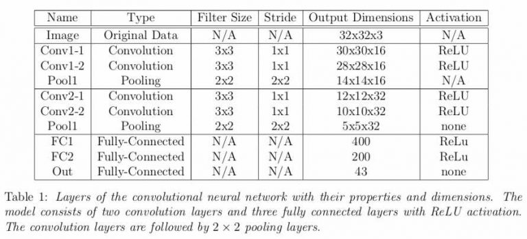
In this project we wrote a convolutional neural network (CNN) image classifier with TensorFlow to distinguish between German traffic signs of the dataset of the German Traffic Sign Recognition Benchmark (GTSRB) challenge. The architecture of the CNN is shown in the table on the bottom right. Convolutional, fully-connected, and pooling layers were used, together with dropout and L2 regularization.
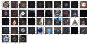
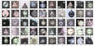
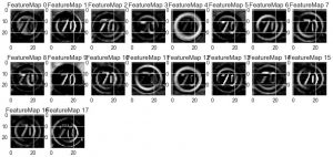
The training dataset was preprocessed and augmented as illustrated on the right, including position and color shifts, as well as masking.
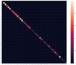
At the end of the training, we reached the following accuracies:
- Training set accuracy: 1.000 (the neural network achieves perfect classification of the training dataset).
- Validation set accuracy: 0.9954
- Test set accuracy: 0.9836
The above result on the test dataset is competitive with some of the top results in the GTSRB challenge, which lie in the 97-99% accuracy range. (It is to be noted though that the format of the competition, which happened several years earlier, was somewhat different, so our results here are not exactly one-to-one comparable.)
The full report for this project is available upon request.
Object Detection (Example: Vehicles on Road)
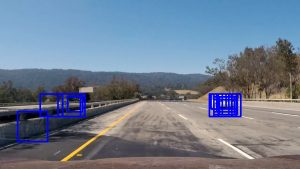
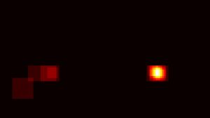
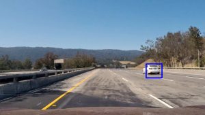
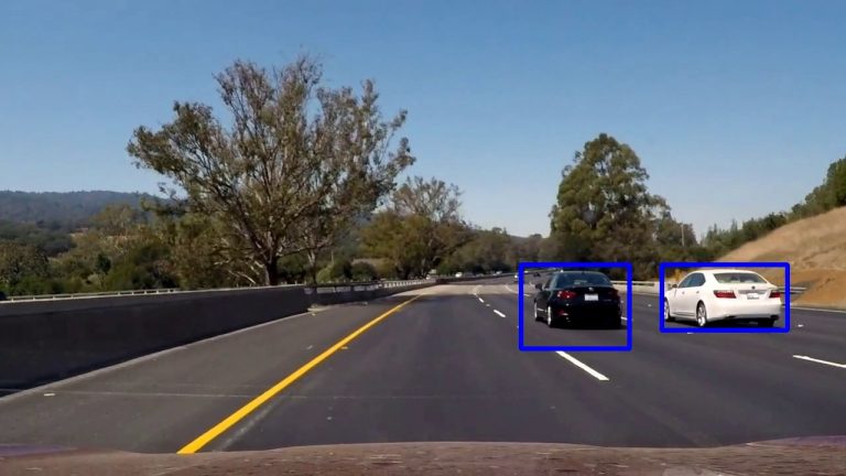
Visual detection of potential obstacles – and in particular other moving vehicles which can never be registered in a static map – is of utmost importance to prevent collisions. In the video on the right, we have implemented a sliding window search coupled with a support vector machine (SVM) classifier to detect cars on a road. The feature vector fed into the SVM came from the histogram of gradients (HOG) combined with a histogram of colors as well as raw color pixel values in HSV and HLS color spaces.
Behavioral Cloning
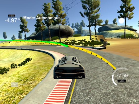
On the right wrote a convolutional neural network (CNN) with Keras in Python and trained it to drive a car on a simulated curvy mountain road.
First we trained the CNN on images and associated steering angles recorded as we drove the car manually for a couple of laps. After this training – and adjustments to the CNN’s architecture -, the CNN was able to drive the car on its own. (The training was done in opposite direction around the track to make sure the CNN did not just remember specifics of the scenery during the training laps).
The CNN achieves this performance alone in this example, without assistance from additional computer vision techniques like lane line finding. A kinematic model of the car, MPC, etc. could also be added to improve performance.
Above: A multi-layer convolutional neural network (CNN) using convolutional, pooling, and fully-connected layers with drop-out and regularization drives a car autonomously on a mountain road in Udacity‘s simulator provided with their Self-Driving Car Engineer Nanodegree program.
Visual Path Detection (Example: Lane Line Finding)
Lane line finding is an obvious computer vision method with which we can strongly augment the performance of the above CNN (though by itself this method may be prone to failure if on some road there are no lane lines).
In the project illustrated on the right, first we calibrated the camera on a checkerboard test image to determine the lens distortion, which was then removed from the individual video frames.
Then lane lines were detected as in the second pair of images on the right. The left image is a sample frame from the original video; in the right image pixels were selected by gradient detection (red), white and yellow pixels found in HSV color space (green), and the thresholded S channel from the HSL color space (blue). A mask was also applied, as illustrated by the overlaid blue trapezoid in the original image; pixels outside the trapezoid were ignored, as lane lines are not supposed to occur there.
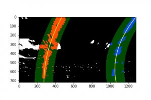
With a perspective transform we converted the image afterwards into what the road would essentially look like in a top-down view (see warped image on the right). This allowed us to fit a second order polynomial to the detected lane line pixels using the sliding window method if no previous lane line was detected, or based on a search around the lane lines found in a previous frame of the video if available. The curvature radius of the lane lines and the position of the car with respect to the center of the lane was determined based on the polynomials and annotated in the individual frames of the video at the bottom. This enables the car to understand its position in the lane explicitly as well as how much the lane is turning (which can be exploited for better driving performance using, for instance, a kinematic model of the car and model predictive control (MPC)).

