Data Science and Computing with Python for Pilots and Flight Test Engineers

Introduction

Let us review briefly what we did at the end of the lesson System Response in the Time Domain. There we had a system defined by differential equation

$$ \ddot x(t) + 2 \dot x(t) + 17 x(t) = f(t) $$

and we chose the input function \(f(t)\) to be a sinusoidal function with just one angular frequency \(\omega=3\) and constant amplitude equal to 1, i.e. the function was \(f(t)=\sin(3t)\). The output of the system \(x(t)\) looked like the plot below, where the red curve depicts the input function \(f(t)\), whereas the blue curve denotes the system response \(x(t)\) to this input function \(f(t)\).

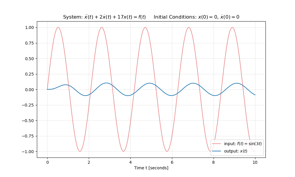
As we can see from the above, the amplitude of the output is different than the input (the output amplitude is much smaller than the input in this case). This ratio of output to input amplitude is called the magnitude or (especially if given in decibel) the gain of the system. We also note that at any given time, the output is at a different point in its wave cycle than the input and that the peaks of the output are somewhat shifted to the right compared to the corresponding peaks of the input. The difference in phase at any given time is called the phase shift, and the time delay observed in the plot above is called the phase delay.

In this lesson, we will learn how to determine from the transfer function of the system the gain, the phase shift, and the phase delay of the output for a sinusoidal input of a given angular frequency \(\omega\). In the next lesson, we will plot these systematically for all possible frequencies \(\omega\) and will thereby arrive at the so called Bode plots.

Magnitude/Gain and Phase Shift

The transfer function for the above system has been shown in previous lessons to be

$$ H(s):=\frac{X(s)}{F(s)} = \frac{1}{s^2+2s+17} $$

This is a complex function of complex variable \(s = \sigma + i\omega\) in the Laplace domain.

Magnitude and Gain

For a sinusoidal input \(f(t)=\sin(\omega t)\) of constant amplitude and angular frequency \(\omega\) we can obtain the ratio of output amplitude to input amplitude by computing the magnitude of this function in the complex plane, if we set \(s=i\omega\):

$$M(\omega):= |H(i\omega)|=\left|\frac{1}{(i\omega)^2+2(i\omega)+17}\right|. $$

The gain in decibel (dB) is defined as

$$ gain[dB](\omega) = 20 \log_{10} M(\omega).$$

Phase Shift

Similarly, we can obtain the phase shift from the argument (angle) of this complex number (angle in the complex plane compared to the positive real axis), also when setting \(s = i\omega\):

$$\phi(\omega) := \arg(H(i\omega)) = \arg\left(\frac{1}{(i\omega)^2+2(i\omega)+17}\right) $$

A negative phase shift means a delay, a positive phase shift means the output is ahead of the input.

Phase Delay

The phase delay is the time difference between the arrival of an output peak and an input peak (or any other specified part of the sine wave). It can be computed from the phase shift above and the angular frequency \(\omega\), and is defined as

$$ \tau_{\phi}(\omega) := – \frac{\phi(\omega)}{\omega} $$

It is defined such that, if \(\tau_{\phi}\) is positive, there is a delay, i.e. the output is behind the input, whereas a negative time delay would mean that the wave of the output is ahead of the input. (One can easily remember this sign convention, as it is the same for the times of athletes arriving at the finish line of a sporting event: if the time difference indicated is positive, the athlete is behind the leader of the race.)

The Code

The function evaluate_transfer_function() below implements the calculation of all of the above. Its arguments are a system \(sys\) and the complex variable \(s\) of the Laplace domain (s-plane), for which in this case we are supposed to set \(s=i\omega\). The output of the function is the value of the transfer function for the supplied value of \(s\), the magnitude (gain), the gain in dB (decibel), the phase shift in rad, the phase shift in degrees, and lastly the phase delay.

import numpy as np
import matplotlib.pyplot as plt

from scipy import signal

def evaluate_transfer_function(sys, s):
    """ Evaluates transfer function H(s) at s and returns:
    complex value of H(s) at s, |H(s)|, arg(H{s}) in rad, arg(H(s)) in deg. """
    numerator = sys.num
    denominator = sys.den
    n = 0.0
    d = 0.0
    
    j = numerator.shape[0]
    for i in range(0, numerator.shape[0]):
        j -= 1
        n = n + numerator[i] * (s**j)

    j = denominator.shape[0]
    for i in range(0, denominator.shape[0]):
        j -= 1
        d = d + denominator[i] * (s**j)

    # Complex value of transfer function at the selected s:        
    tf = n/d

    magnitude = np.abs(tf)
    gain = 20.0 * np.log10(magnitude)

    angle = np.angle(tf)
    time_delay = - angle / s.imag
    
    return tf, magnitude, gain, angle, angle/(2.0*np.pi)*360.0, time_delay

To apply this function for the specific case above, we first create the corresponding system:

omega = 3
sys = signal.TransferFunction([1],[1,2,17])

Then we apply the function to this system and \(s=3i\), we obtain the following output:

transfer_function_value, magnitude, gain_dB, phase_shift_rad, phase_shift_deg, phase_delay = evaluate_transfer_function(sys, omega*1j)

((0.08-0.06j), 0.1, -20.0, -0.6435, -36.8699, 0.2145)

We see that the magnitude is 0.1 (which is -20 in dB), the phase shift is -36.8699 degrees, and the phase delay is 0.2145 seconds.

In the next lesson, we plot the gain and the phase shift systematically for all angular frequencies \(\omega\) (Bode plot) and thereby get information about the whole frequency response of the system.