Data Science and Computing with Python for Pilots and Flight Test Engineers

In this section we will learn how to perform geometric camera calibration and distortion correction. (The geometric camera calibration discussed in this lesson is not to be confused with photometric camera calibration, which deals with the brightness of the color channels of individual pixels and thus ultimately with the recording and rendering of colors in images).

From calibration images containing a chessboard (an illustration can be found at the very bottom of this page), we will infer parameters of our optical system by computing the camera matrix and the distortion coefficients. From these we will able to determine optical system parameters such as focal length, which will allow us to transfer measurements in the 2D image to measurements of angles and lengths in the 3D world, of which the image was taken. This is important for scene understanding.

No optical system is perfect. Images taken by a real world optical system have distortions. Knowing the camera matrix and the distortion coefficients will also allow us to correct for these distortions and undistort the images. This is important before we make measurements, because distortions make objects appear in different pixels than they should, and this measurement error in our 2D image would translate to incorrect conclusions about the 3D world.

Much of the material presented here, including some of the code, comes from the Camera Calibration section of the OpenCV open source computer vision library documentation. The reader is highly encouraged to consult this documentation for an explanation of the theory. Below, for now, we focus merely on how to do it.

import matplotlib.pyplot as plt
import matplotlib.image as mpimg
import numpy as np

import cv2
import glob
from itertools import product

import copy

%matplotlib inline

Camera Calibration: Computing Camera Matrix and Distortion Coefficients

In this section we computer the camera matrix and distortion coefficient form a set of calibration images containing a chessboard. The chessboard corner detection function was mostly taken from the Camera Calibration section of the OpenCV documentation, with small modifications.

def obtain_calibration_image_names(path):
    """ Make a list of file names of the calibration images. """
    image_names = glob.glob(path + 'calibration*.jpg')
    return image_names

def perform_calibration_point_detection(calibration_image_names):
    """ Maps object points in 3D to image points in 2D from chessboard calibration images. """

    # termination criteria for point refinement
    criteria = (cv2.TERM_CRITERIA_EPS + cv2.TERM_CRITERIA_MAX_ITER, 30, 0.001)

    # Arrays to store object points and image points from all the images.
    objpoints = [] # 3D points in real world space
    imgpoints = [] # 2D points in image plane

    for image_name in calibration_image_names:

        print("Reading Calibration Image:", image_name)
        img = cv2.imread(image_name)
        gray = cv2.cvtColor(img, cv2.COLOR_BGR2GRAY)
        image_dimensions = gray.shape[::-1] # gets width and height; use .shape[1::-1] if based on a color image.
        
        # Run through different numbers of detected corners (adjust as needed):
        for corners_width, corners_height in product(range(10,7,-1), range(6,4,-1)): 

            # prepare object points, like (0,0,0), (1,0,0), (2,0,0) ....,(6,5,0)
            objp = np.zeros((corners_height*corners_width, 3), np.float32)
            objp[:, :2] = np.mgrid[0:corners_width, 0:corners_height].T.reshape(-1,2) # x, y coordinates
            # z coordinate always zero, because chess board is fixed in space in (x,y)-plane (z=0).

            # Find the chess board corners:
            ret, corners = cv2.findChessboardCorners(gray, (corners_width,corners_height), None)
            print("Found Corners (dims", corners_width, ",", corners_height ,"):", ret)

            # If found, add object points, image points (after refining them)
            if ret == True:
                objpoints.append(objp)

                corners2 = cv2.cornerSubPix(gray,corners, (11,11), (-1,-1), criteria)
                imgpoints.append(corners2)
                
                # Draw and display the corners:
                img = cv2.drawChessboardCorners(img, (corners_width,corners_height), corners2, ret)
                img = cv2.cvtColor(img, cv2.COLOR_BGR2RGB)
                plt.imshow(img)
                plt.show()

                break # break out of double loop if correct corner number detected.

    return objpoints, imgpoints, image_dimensions
    
    

def compute_camera_calibration(objpoints, imgpoints, calibration_dimensions):
    """ Computes camera matrix and distortion coefficients. """
    ret, camera_matrix, distortion_coefficients, rvecs, tvecs = cv2.calibrateCamera(objpoints, imgpoints, calibration_dimensions, None , None)
    return ret, camera_matrix, distortion_coefficients, rvecs, tvecs

Now that we have all the required functions, run the actual calibration:

calibration_image_path = './Camera Calibration/camera_calibration_images/camera_calibration_images_Udacity/'
cal_image_names = obtain_calibration_image_names(calibration_image_path)
objpoints, imgpoints, calibration_image_dims = perform_calibration_point_detection(cal_image_names)
ret, camera_matrix, distortion_coefficients, rvecs, tvecs = compute_camera_calibration(objpoints, imgpoints, calibration_image_dims)

Now we have the camera matrix and distortion coefficients, which contain the parameters of our optical system. We will also use them to undistort images taken with this optical system. This is done in the next section.

Image Distortion Correction

def perform_distortion_correction(original_image, camera_matrix, distortion_coefficients):
    """ Correct the distortion of an image, using the known camera matrix and distortion coefficients of the system (obtained during camera calibration). """
    undistorted_image = cv2.undistort(original_image, camera_matrix, distortion_coefficients, None, camera_matrix)
    return undistorted_image

Perform the distortion correction on a sample image, by applying the camera matrix and distortion coefficients we have computed in the code cells in the previous section.

original_image = mpimg.imread('./original_image.jpg')

undistorted_image = perform_distortion_correction(original_image, camera_matrix, distortion_coefficients)

plt.imshow(original_image)
plt.show()
plt.imshow(undistorted_image)
plt.show()

Plot the Comparison of Original Image and Undistorted Image

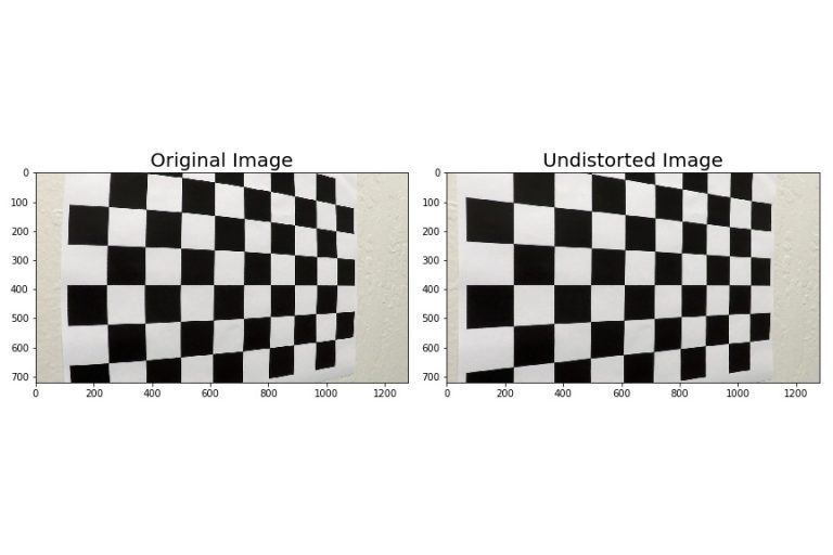
With the simple code below, we display a side by side comparison of the original image and of the undistorted one. The lines of the chessboard in the undistorted image are clearly straighter than in the original one, especially on the left-hand side of the board, which is closer to the viewer.

def side_by_side_plot(image1, image2, title1, title2, filename=None):

    f, (ax1, ax2) = plt.subplots(1, 2, figsize=(20, 10))
    f.tight_layout()

    ax1.imshow(image1)
    ax1.set_title(title1, fontsize=30)

    ax2.imshow(image2)
    ax2.set_title(title2, fontsize=30)
    plt.subplots_adjust(left=0., right=1, top=0.9, bottom=0.)
    plt.tight_layout()
    if filename is not None:
        plt.savefig(filename)
    plt.show()

side_by_side_plot(original_image, undistorted_image, 'Original Image', 'Undistorted Image', './original_and_undistorted_image.jpg')

Note that in both images the lines still show perspective, because one end of the board is closer to the camera than the other. This is normal and desired; it is supposed to look that way. The removal of perspective from an image before certain measurements is the topic of the perspective transform covered in a separate lesson. This section here deals only with image distortions that come from the imperfections of the optical system (e.g. barrel and pincushion distortion) and, for instance, make some lines appear curved in the image, where in fact they should be straight.