Data Science and Computing with Python for Pilots and Flight Test Engineers

Introduction

While many of our lessons in this course are code oriented, this lesson will further your physical intuition of the kind of systems we are dealing with, and it will increase your ability to solve these kinds of problems analytically.

The mass-spring-damper system treated here is simple example of a second-order physical system illustrating the behavior of systems obeying an equation of motion of the type

\begin{equation} a\ddot x(t) + b \dot x(t) + c x(t) = f(t) \end{equation}

This system, also called a damped harmonic oscillator, is used as a prototype system from classical mechanics to develop physical intuition, and other such systems are often conceptually referred to this system, even if their underlying physics is entirely different. For instance, when we discuss the short period mode of longitudinal dynamic stability of an aircraft or the Dutch roll mode of lateral-directional dynamic stability, we will ask ourselves, which term in their equations of motion is the “spring” term and which is the “damping” term, even though there is no physical spring present on the aircraft in either of these cases.

Description of the Mass-Spring-Damper System

The mass-spring-damper system comprises a block of mass sliding on a frictionless surface (or rolling on frictionless wheels with zero moment of inertia), a spring which is attached to it on one side, and a damping device, which creates a force opposite to any motion and which is proportional to the velocity of the block of mass. The position of the block of mass is described by variable \(x(t)\). The position where the spring does not exert any force is at \(x=0\). This is illustrated in the image below.

This mass-spring-damper system obeys the physical differential equation of motion

$$ m\ddot x(t) + d \dot x(t) + k x(t) = f(t), $$

where \(m\) is the mass of the block, \(k\) is the spring constant, and \(d\) (often called \(c\) in other sources) is the damping constant.

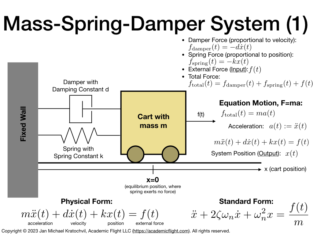
From a systems point of view, we can consider the external force \(f(t)\), that we can let act on the mass, if we wish, as the input function of the system, and the position of the mass \(x(t)\) as the output of the system ((\(x(t) \) is also part of the state vector of the system, together with \(\dot x(t)\)).

Equation of Motion in Standard Form

It will turn out be convenient to rewrite the above equation in such a fashion that replaces the physical parameters \(m\), \(d\), \(k\), and \(f(t)\) above with other parameters that yield information about the shape of the solutions of the system. To this end, we divide the whole equation by mass \(m\) and perform a few other variable replacements, by introducing the natural frequency parameter \(\omega_n\) and damping ratio \(\zeta\), as is illustrated in the slide below. The new parameters \(\omega_n\) and \(\zeta\) can be obtained easily from the original parameters, so no difficult calculation is necessary. The differential equation now takes the standard form

$$ \ddot x(t) + 2 \zeta\omega_n \dot x(t) + \omega_n^2 x(t) = \frac {f(t)}{m}. $$

Computing the Solution

Let us now compute an analytic solution of this standard equation of motion

$$ \ddot x(t) + 2 \zeta\omega_n \dot x(t) + \omega_n^2 x(t) = \frac {f(t)}{m}. $$

with the tools we have learned so far, for the free response of the system to a unit impulse \(f(t)/m=\delta(t)\) and zero initial condition. This means, the system is at equilibrium at rest, and something briefly excites it. We want to see how the system responds.

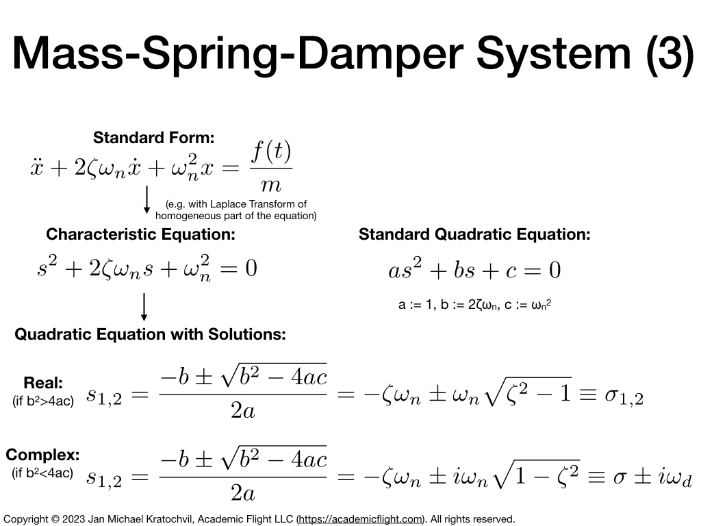
To compute the solution, we perform a Laplace transform of the whole equation first and obtain

$$ s^2 X(s) + 2 \zeta\omega_n s X(s)+ \omega_n^2 X(s) = \frac {F(s)}{m} = \delta(s)$$

The transfer function is

$$ H(s) = \frac{X(s)}{\delta(s)} = \frac{1}{s^2 + 2 \zeta\omega_n s + \omega_n^2}. $$

The solution in the Laplace domain is \(X(s) = H(s)\delta(s) = H(s)\), because we remember from the Laplace transformation lesson that the Laplace transform of the unit impuls, \(\delta(s)=1\).

In order to obtain the solution in the time domain, we must now perform the inverse Laplace transform of solution \(X(s)\) in the Laplace domain

$$ X(s) = \frac{1}{s^2 + 2 \zeta\omega_n s + \omega_n^2}. $$

Performing the Inverse Laplace Transform

The method we advocated to perform the inverse Laplace transform to obtain \(x(t)\), was to write the function \(X(s)\) as a sum of terms, each of which we can recognize as known Laplace transforms of functions in the table of Laplace transforms, which we presented in the lesson on Laplace Transforms.

Case 1: Denominator has Two Distinct Real Roots

Let us assume that the second order polynomial in the denominator of \(X(s)\) above has two distinct real roots \(\sigma_1\) and \(\sigma_2\). Then \(s^2 + 2 \zeta\omega_n s + \omega_n^2 = (s-\sigma_1)(s-\sigma_2)\). (We can compute \(\sigma_1\) and \(\sigma_2\) in terms of \(\zeta\) and \(\omega\) with the standard formula for quadratic equations, as is illustrated in the slide below (real case), to obtain values for them, if we want.)

We then perform partial fraction decompostion to write the solution as a sum of terms for which we know the Laplace transforms

$$ \frac{1}{(s-\sigma_1)(s-\sigma_2)} = \frac{A}{s-\sigma_1} + \frac{B}{s-\sigma_2}$$

This can be also written as

$$ \frac{1}{(s-\sigma_1)(s-\sigma_2)} = \frac{A(s-\sigma_2)}{(s-\sigma_1)(s-\sigma_2)} + \frac{B(s-\sigma_1)}{(s-\sigma_1)(s-\sigma_2)}$$

Setting \(s=\sigma_1\) yields \(1=A(\sigma_1-\sigma_2)\) and thus \(A = \frac{1}{\sigma_1-\sigma_2}\). Likewise, setting \(s=\sigma_2\) yields \(1=B(\sigma_2-\sigma_1)\) and thus \(B = \frac{1}{\sigma_2-\sigma_1}=-A\).

Therefore, we obtain

$$ X(s) = \frac{1}{(\sigma_1-\sigma_2)(s-\sigma_1)} + \frac{1}{(\sigma_2-\sigma_1)(s-\sigma_2)} = \frac{1}{\sigma_1-\sigma_2}\left(\frac{1}{s-\sigma_1} – \frac{1}{s-\sigma_2}\right) $$

We recognize the last two terms as the Laplace transform \(\frac{1}{s+\sigma}\) of the exponential function \(e^{-\sigma}\) in the table, with \(\sigma=-\sigma_1\) and \(\sigma=-\sigma_2\).

The analytic solution of the differential equation in the time domain in Case 1 is therefore

$$ x(t) = \frac{1}{\sigma_1-\sigma_2} (e^{\sigma_1t}-e^{\sigma_2t}) $$

with, as we mentioned earlier, \(\sigma_{1,2} = -\zeta\omega_n \pm \omega_n \sqrt{\zeta^2-1}\) computable with the standard quadratic formula.

Case 2: Denominator has Two Identical Real Roots

When the denominator of the solution in Laplace domain, \(X(s)\) has two identical real roots, this leads to a different partial fraction decomposition, if you recall from our inverse Laplace transform lesson. Thus, this leads to different Laplace transforms of functions, ultimately resulting in different analytic solutions in the time domain. We leave this as an exercise to the reader, it is analogous to the above and fairly similar. You will have an opportunity to verify your solutions by comparison to the numerical one at the end of this lesson.

Case 3: Denominator has No Real Roots (Complex Conjugate Pair)

If the denominator of the solution in Laplace domain, \(X(s)\), has no real roots at all, but instead a complex conjugate pair, this again needs to be treated differently in the partial fraction decomposition, before the inverse Laplace transform. The functions which we will now be able to identify in the Laplace transform are the damped sine and cosine waves. This is also left as an exercise to the reader. When you calculate it, do the cosine first, and then the sine; it works better that way. Below you can see what your result should look like (with constants \(A\) and \(B\) still for you to be determined, e.g. from the initial conditions at time \(t=0\)).

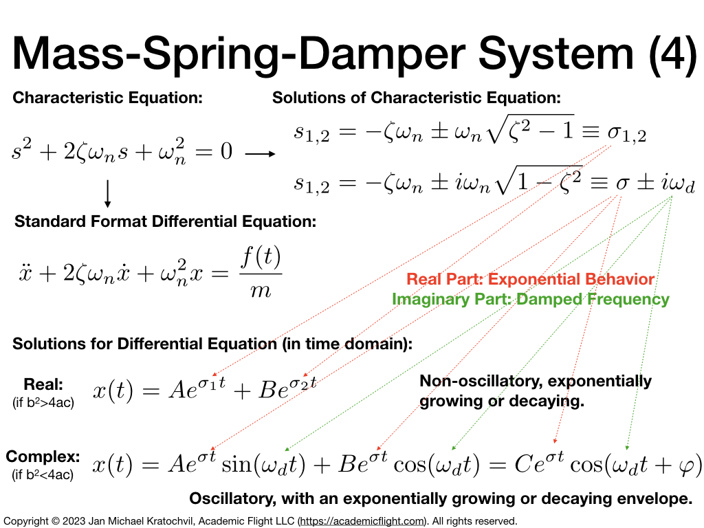
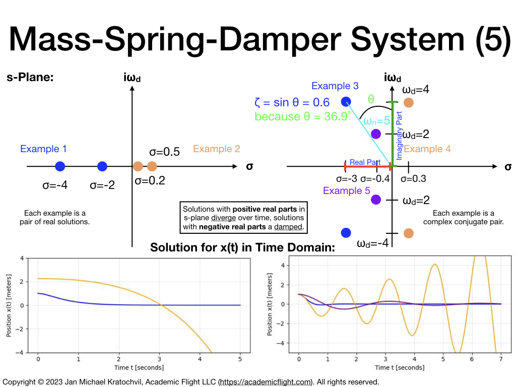
We can plot these analytic solutions and obtain the plots below. We also show how the parameters of these solutions and of the differential equation in standard form can be identified in the \(s\)-plane with the locations of the poles of the solution \(X(s)\). Solutions with poles in the left half of the \(s\)-plane are damped and converge to the equilibrium position (at \(x=0\)), while solutions with at least one pole in the right half of the \(s\)-plane grow with time. Solutions with real poles decay or grow exponentially without oscillating (they are called over-damped), while solutions with complex conjugate pairs of poles decay or grow while being oscillatory.

Comparison between Analytic and Numerical Solutions

Above we have obtained the solution for \(x(t)\) analytically, by performing the Laplace transforms by hand and obtaining a closed-form solution. In this section, we want to compare this solution to the numerical solution we can obtain with the scipy.signal or control.matlab submodules, which we have learned how to use.

Case 1

To study an example case with two real roots in the denominator of the solution \(X(s)\) in the Laplace domain, let us set \(\zeta=2\) and \(\omega_n=5\) in equation

$$ \ddot x(t) + 2 \zeta\omega_n \dot x(t) + \omega_n^2 x(t) = \frac{f(t)}{m}. $$

and obtain the solution \(x(t)\) for a unit impulse \(f(t)/m=\delta(t)\). We can then compare our analytic solution obtained above

$$ x(t) = \frac{1}{\sigma_1-\sigma_2} (e^{\sigma_1t}-e^{\sigma_2t}) $$

with

$$ \sigma_{1,2} = -\zeta\omega_n \pm \omega_n \sqrt{\zeta^2-1}$$

to our numerical solution from the scipy.signal submodule, using the following code:

import numpy as np
import matplotlib.pyplot as plt

from scipy import signal

zeta = 2
omega_n = 5

# Analytic solution: (case with two real roots)
sigma1 = - zeta*omega_n + omega_n * np.sqrt(zeta**2 - 1)
sigma2 = - zeta*omega_n - omega_n * np.sqrt(zeta**2 - 1)

t_analytic = np.linspace(0, 5, 1001)
x_analytic = 1.0/(sigma1-sigma2)*(np.exp(sigma1*t_analytic)-np.exp(sigma2*t_analytic))

# Numerical solution:
sys = signal.TransferFunction([1],[1, 2*zeta*omega_n, omega_n**2])
t, x = signal.impulse(sys)

# Plot x(t):
plt.plot(t_analytic, x_analytic, color="tab:red", label="Analytic Solution")
plt.plot(t, x, color="tab:blue", label="Numerical Solution")
plt.xlabel('t [seconds]')
plt.ylabel('x(t)')
plt.legend()
plt.show()

Run this code above at home in your Jupyter notebook and observe, how well the two solutions agree.

Case 2

Now please do the same for Case 2. As an example, pick values \(\zeta = 1\) and \(\omega_n=5\). This will provide a means for you to check, if you obtained the correct analytic solutions for these two cases.

Case 3

For Case 3, you can choose \(\zeta = 0.5\) and \(\omega_n=5\). This will result in a complex conjugate pair of roots (no real ones) for the denominator of \(X(s)\).