Data Science and Computing with Python for Pilots and Flight Test Engineers

Introduction

There are many ways to solve a differential equation, and different forms of differential equations lend themselves better to some solution procedures than others. The type of equation we will be dealing with mostly in this part of the course will be a linear ordinary differential equation with constant coefficients. In general, such an equation has the form

\begin{equation} a_n x^{(n)}(t) + a_{n-1} x^{(n-1)}(t) + a_{n-2} x^{(n-2)}(t) + \dots + a_2\ddot x(t) + a_1 \dot x(t) + a_0 x(t) = f(t), \end{equation}

where \(x^{(n)}(t) \) denotes the \(n\)-th time derivative of \(x(t)\) (in principle, it should be denoted with \(n\) dots above the letter \(x\), but there was not enough space. We can think of \(f(t)\) as the input function into some system (e.g. a signal input), and the solution \(x(t)\) of the above equation as the output function (e.g. a signal output) of the system described by the differential equation.

Oftentimes we will only have derivatives up to order \(n=2\), sometimes even only \(n=1\), but we wanted to include the higher derivatives as well, because the solution described below works for all these cases.

Solving a Differential Equation using the Laplace Transform

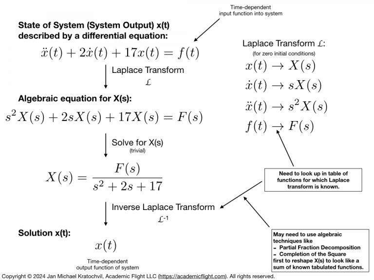
The solution we outline here – and will explain in further lessons – is illustrated in the slide below. The differential equation (in the time domain), which is a challenge to solve, is first subjected to a Laplace transform (which we will discuss in the next lesson). The Laplace transform turns the equation into an algebraic equation in the Laplace domain, which we can very easily solve. But the solution we obtain is, of course, still in the Laplace domain. Therefore, we need to apply the inverse Laplace transform to this solution to obtain the desired solution of the equation in the time domain.

We have thus turned the solution of a differential equation into a simple solution of an algebraic equation. But how do we compute the two Laplace transforms? We will simply look them up in a table (for known functions, for which the Laplace transform has been tabulated).

The reader sees that this is not some magic easy way to solve the differential equation without any work; someone had to put in some real effort to compute the Laplace transforms for a whole bunch of functions and put them into a table. The point is, it was not us! And we do not even particularly care, how they were computed. We can just use them from the table, and thus defer the problematic of solving the differential equation to a simple table lookup.

The only challenge that we will have sometimes, is that a function will not always look initially like any of the equations in the lookup table of Laplace transforms. We will then have to use some benign algebraic techniques, such as partial fraction decomposition and completing the square, in order first to write the function as a sum of terms, for each of which we can find the Laplace transform tabulated. This process will become especially relevant for the inverse Laplace transform, because the solution of our differential equation in the Laplace domain will be some rational function in the complex variable \(s\). The fraction will have to be broken into some more manageable pieces, and the individual pieces perhaps a bit reshaped. (For the forward transform, \(f(t)\) is typically chosen to be a function that has been tabulated, and the Laplace transforms of the derivatives of \(x(t)\) are already in the Laplace transform lookup table.