Data Science and Computing with Python for Pilots and Flight Test Engineers

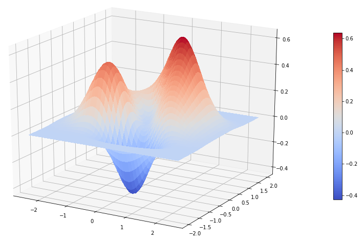
In the previous lesson we have seen how to plot the graph of a function of two variables as a contour plot, where the value of the function was represented by color. We can also visualize the same plot in 3D.

We can quickly proceed to making 3-dimensional plots as well. While this is a bit more involved, you can again just copy and paste the code and modify it for your purposes by plotting a different function or changing the view point.

import numpy as np
import matplotlib.pyplot as plt

# 3D surface plots require us to import parts of additional modules: 
from mpl_toolkits import mplot3d
from matplotlib import cm

def function2(x, y):
    z = (x**2 + x*y + y**3) * np.exp(-(x**2 + y**4)) # this is the equation of the function we are plotting in this example.
    return z

# This creates a 2D grid of points where the function will be evaluated for plotting.
x = np.linspace(-2.5, 2.5, 100)
y = np.linspace(-2, 2, 100)
x, y = np.meshgrid(x, y)
 
# This assigns the values of function "function2" on that grid to variable z: 
z = function2(x, y)

# Now create the surface plot:

# Set up the figure:
fig = plt.figure(figsize=(15,10))
# Set up the axes for figure:
ax = fig.add_subplot(111, projection='3d')

# Make the 3D plot, plotting the function as a 2D surface in 3D:
surf1 = ax.plot_surface(x, y, z, rstride=2, cstride=2, cmap=cm.coolwarm, linewidth=0, antialiased=False)

fig.colorbar(surf1, shrink=0.6, aspect=20) # optionally adds color bar on the right. 

# Optionally, adjust viewing position from which you view the surface: elevation, azimuth, and distance:
ax.elev = 20.0
ax.azim = -60.0
ax.dist = 10.0

plt.savefig("./surface_plot_in_3D.png") # optionally save the plot to a file on your hard drive.

plt.show()

Copy and paste the above code into a Jupyter notebook on your computer to create your first amazing 3D surface plot.