Data Science and Computing with Python for Pilots and Flight Test Engineers
System Response in Time Domain
In this lesson we will find solutions \(x(t)\) of the state or output of the system in the time domain, i.e. as a function of time, for different inputs \(f(t)\). First we will look at two fundamental standard inputs, the unit impulse and the unit step, and then we will consider an arbitrary input \(f(t)\).
We emphasize that these solutions are in the time domain, which is in contrast to finding solutions in the Laplace domain (s-plane), where we would find the Laplace transform \(X(s)\) of \(x(t)\). Computing our task here by hand, one would find \(X(s)\) first and then perform an inverse Laplace transform to obtain \(x(t)\). The computer does all of this for us, of course, so the code below outputs \(x(t)\) of the system directly, given an input function \(f(t)\). Initial conditions are assumed to be zero (but this can be generalized easily).
Time Domain Solutions with scipy.signal Submodule of SciPy Library
Let us once again create a system with differential equation
$$ \ddot x(t) + 2 \dot x(t) + 17 x(t) = f(t) $$
which (assuming zero initial conditions, as we have seen in previous lessons) has transfer function
$$ H(s) := \frac{X(s)}{F(s)} = \frac{1}{s^2+2s+17}. $$
\(s\) here is the variable in Laplace domain (complex valued frequency domain), and \(X(s)\) and \(F(s)\) are the Laplace transforms of \(x(t)\) and \(f(t)\), respectively.
As usual can create an instance of such a system, for example, in transfer function representation with one line of code:
import numpy as np
import matplotlib.pyplot as plt

from scipy import signal
sys = signal.TransferFunction([1], [1,2,17])Below we will look at three different forcing functions \(f(t)\) and we will find solutions \(x(t)\) in the time domain (as opposed to Laplace or Fourier domain). The forcing functions (or input functions) \(f(t)\) which we will consider are the unit impulse input, \(\delta(t)\) (Dirac delta function), the unit step input, \(\theta(t)\) (Heaviside step function), and an arbitrary function (i.e. a generic solution).
System Response to a Unit Impulse Input (Unit Impulse Response)
A unit impulse input function is the Dirac delta function in the time domain: it is a generalized function which is non-zero only at time \(t=0\), where it is essentially infinitely high, such that the time integral over the whole function equals 1. It symbolizes an infinitely brief, sharp input of 1.
The unit impulse response is the inverse Laplace transform of the transfer function \(H(s)\) of the system. It is obtained by (this works for a system defined in any of the three representations):
t, x = signal.impulse(sys)Let us plot the result. Because it is in the time domain, we have time \(t\) on the horizontal axis.
plt.figure()
plt.plot(t,x)
plt.xlabel("Time t [seconds]")
plt.ylabel("x(t)")   # system output x(t) for impulse input f(t).
plt.grid()
plt.show()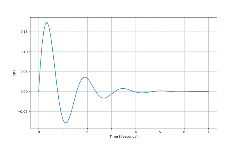
System Response to a Unit Step Input (Unit Step Response)
The unit step input is the next most basic input. It corresponds to a forcing function \(f(t)\) which is zero anytime before time \(t=0\), becomes 1 at \(t=0\) and – unlike the unit impulse input above – remains 1 for all time after that.
t, x = signal.step(sys)Again, a single line of code above gets us the result, and the only thing we still need to do is plot the result:
plt.figure()
plt.plot(t,x)
plt.xlabel("Time t [seconds]")
plt.ylabel("x(t)")   # system output x(t) for impulse input f(t).
plt.grid()
plt.show()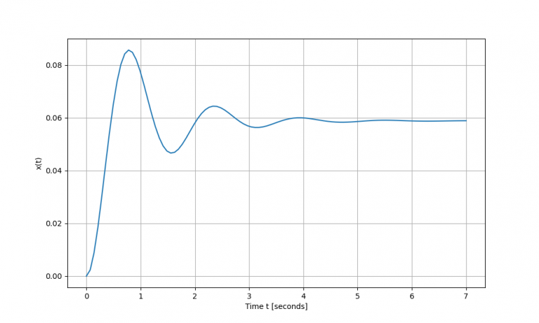
System Response to an Arbitrary Input
In general, of course, the forcing function (input function) \(f(t)\) is an arbitrary function of time. For this case, there is also a convenient way to obtain the output of the system in the time domain. Below we pick the sinusoidal input function \(f(t) = \sin (3t)\) as an example, but this method works for any arbitrary function \(f(t)\).
t = np.linspace(0, 50, 1000)   # points in time to plot input/output functions
u = np.sin(3*t)   # input function f(t)=sin(3t)

tout, yout, xout = signal.lsim(sys, U=u, T=t)
Above, \(xout\) is time evolution of the state vector, \(yout\) is time evolution of the output vector, and \(tout\) contains the list of computed output times.
plt.figure(figsize=(10,6))
plt.plot(t, u, color='tab:red', alpha=0.5, label='input: $f(t)=\sin(3 t)$')
plt.plot(tout, yout, color='tab:blue', label='output: $x(t)$')
plt.grid(alpha=0.3)
plt.xlabel('Time t [seconds]')
plt.title('System: $\ddot x(t) + 2 \dot x(t) + 17 x(t) = f(t)$     Initial Conditions: $x(0)=0$, $\dot x(0)=0$')
plt.legend(loc='lower right')
plt.savefig('./sinusoidal_input_response.png')
plt.show()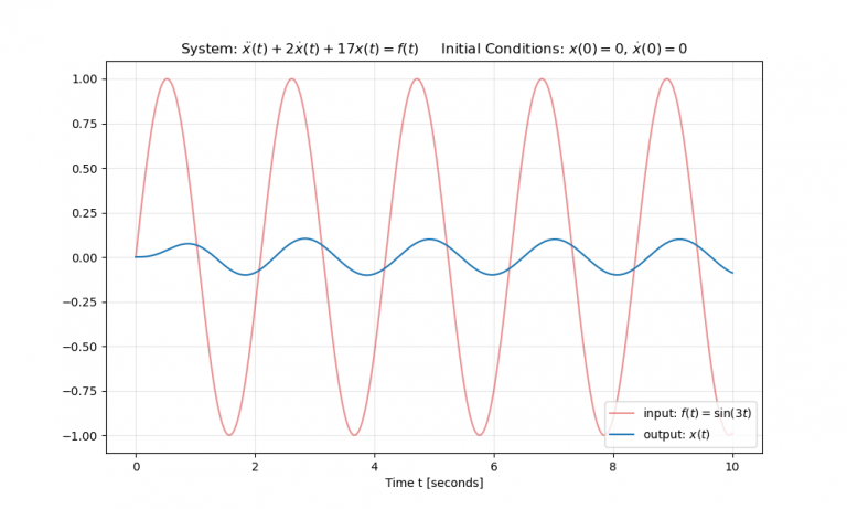
Time Domain Solutions with control.matlab Submodule of python-control Library
Let us once again create a system with differential equation
$$ \ddot x(t) + 2 \dot x(t) + 17 x(t) = f(t) $$
which (assuming zero initial conditions, as we have seen in previous lessons) has transfer function
$$ H(s) := \frac{X(s)}{F(s)} = \frac{1}{s^2+2s+17}. $$
\(s\) here is the variable in Laplace domain (complex valued frequency domain), and \(X(s)\) and \(F(s)\) are the Laplace transforms of \(x(t)\) and \(f(t)\), respectively.
As usual, we can create an instance of such a system, for example, in transfer function representation with one line of code:
import numpy as np
import matplotlib.pyplot as plt

from control.matlab import *
sys = tf([1],[1,2,17])Below we will look at three different forcing functions \(f(t)\) and we will find solutions \(x(t)\) in the time domain (as opposed to Laplace or Fourier domain). The forcing functions (or input functions) \(f(t)\) which we will consider are the unit impulse input, \(\delta(t)\) (Dirac delta function), the unit step input, \(\theta(t)\) (Heaviside step function), and an arbitrary function (i.e. a generic solution).
System Response to a Unit Impulse Input (Unit Impulse Response)
A unit impulse input function is the Dirac delta function in the time domain: it is a generalized function which is non-zero only at time \(t=0\), where it is essentially infinitely high, such that the time integral over the whole function equals 1. It symbolizes an infinitely brief, sharp input of 1.
The unit impulse response is the inverse Laplace transform of the transfer function \(H(s)\) of the system. It is obtained by (this works for a system defined in any of the three representations):
x, t = impulse(sys_TF)Note that the syntax above is very similar to the scipy.signal module, but the variables in the output of the impulse() function here are in a different order.
Let us plot the result. Because it is in the time domain, we have time \(t\) on the horizontal axis.
plt.figure()
plt.plot(t,x)
plt.xlabel("Time t [seconds]")
plt.ylabel("x(t)")   # system output x(t) for impulse input f(t).
plt.grid()
plt.show()
The output looks the same as for the one obtained earlier with the scipy.signal module, so the plot is not shown here again.
System Response to a Unit Step Input (Unit Step Response)
The unit step input is the next most basic input. It corresponds to a forcing function \(f(t)\) which is zero anytime before time \(t=0\), becomes 1 at \(t=0\) and – unlike the unit impulse input above – remains 1 for all time after that.
x, t = step(sys)Again, a single line of code above gets us the result, and the only thing we still need to do is plot the result:
plt.figure()
plt.plot(t,x)
plt.xlabel("Time t [seconds]")
plt.ylabel("x(t)")   # system output x(t) for impulse input f(t).
plt.grid()
plt.show()
The output looks the same as for the one obtained earlier with the scipy.signal module, so the plot is not shown here again.
System Response to an Arbitrary Input
In general, of course, the forcing function (input function) \(f(t)\) is an arbitrary function of time. For this case, there is also a convenient way to obtain the output of the system in the time domain.
Above, \(xout\) is time evolution of the state vector, \(yout\) is time evolution of the output vector, and \(tout\) contains the list of computed output times.