Straight Gliding Flight

This article deals with straight gliding flight, as it is encountered during an engine-out emergency or in a glider. Controlling (and maximizing) glide distance (or minimizing glide path angle) and airspeed management are of primary concern in this situation. This is in contrast to our article on turning gliding flight (in preparation), where the objective is to minimize altitude loss per degree of turn while distance traveled is either irrelevant or is also desired to be kept small (for instance during the turnback maneuver after engine failure after takeoff). Consequently, the conclusions in these two articles differ correspondingly. The images in this article are featured slides from our flight dynamics ground school.

Physics of Straight Gliding Flight

Force Equations

We shall study the case where the airplane is flying long a straight, descending glide path at constant airspeed with the engine inoperative. This is a straight-line motion at constant speed and therefore unaccelerated. In unaccelerated flight the sum of all forces acting on the aircraft must be zero:

\begin{equation}
\mathbf{L} + \mathbf{D} + \mathbf{Y} + \mathbf{W} + \mathbf{T} = \mathbf{0}
\end{equation}
where $\mathbf{L}$ denotes lift, $\mathbf{D}$ denotes drag, $\mathbf{Y}$ denotes side force (all of which are pointing along one of the axes of the wind frame $\mathcal{W}$), $\mathbf{W}$ denotes weight force (pointing along the $z_\mathcal{E}$-axis of the inertial frame) and $\mathbf{T}$ denotes thrust, taken for simplicity to point along the $x_\mathcal{B}$-axis of the body frame $\mathcal{B}$ of the aircraft.

In power-off gliding flight, thrust is zero, $\mathbf{T}=\mathbf{0}$. If the airplane is not flying in a sideslip, sideforce $\mathbf{Y}$ is also zero. So the remaining equation (really a vector equation consisting of three scalar equations) reads
\begin{equation}
\mathbf{L} + \mathbf{D} + \mathbf{W} = \mathbf{0}
\end{equation}
We shall also assume that there is no wind blowing over the earth surface, i.e. the air is at rest in the inertial frame $\mathcal{E}$.

We shall now proceed to write this equation in components in the wind frame $\mathcal{W}$ of the aircraft, resulting in three scalar equations. Along the $y_\mathcal{W}$-axis there are no forces and this equation is trivially zero. We are left with only the $x_\mathcal{W}$- and the $z_\mathcal{W}$-axis equations. A quick peek at the force vector diagram reveals that, with $\gamma$ denoting the glide path angle
\begin{eqnarray}
D &=& – W \sin \gamma\\
L &=& W \cos \gamma.
\end{eqnarray}
As usual, we use the notation $D=|\mathbf{D}|$, $L=|\mathbf{L}$, and $W=|\mathbf{W}|$ for the magnitudes (lengths) of the force vectors. The minus sign in the first equation comes from the fact that downwards flight path angles are negative. Also, do not confuse the magnitude of the weight force vector $W=mg$ with the symbol for the wind frame $\mathcal{W}$, which is typeset in calligraphic font ($m$ is the mass of the aircraft, while $g$ denotes the gravitational acceleration of the earth near the earth’s surface).

We shall now obtain expressions for the glide path angle $\gamma$ and for airspeed $V=|\mathcal{V}|$ in gliding flight from these two force equations.

Glide Path Angle and Glide Distance

Let us point out first that knowing the initial altitude of the aircraft above ground and the glide path angle $\gamma$ leads us to knowing the glide distance from that altitude. So while a pilot is usually more interested in glide distance in case of an emergency, studying the glide path angle $\gamma$ here reveals the same insights: the smaller the glide path angle $\gamma$, the larger the glide distance from any given altitude. In particular, if we will want to maximize glide distance, we will have to minimize glide path angle $\gamma$.

So let us obtain a general expression for $\gamma$ first. Dividing the above two equations by each other (each side), and remembering from trigonometry that $\tan \gamma=\sin \gamma/\cos \gamma$ for any angle $\gamma$, we obtain
\begin{equation}
\tan \gamma = -\frac{D}{L}= -\frac{C_D}{C_L}.
\end{equation}
In the last step we have used the definitions for coefficients of lift, $C_L$, and drag, $C_D$, respectively:
\begin{eqnarray}
L &=&\frac{1}{2}\rho V^2 S C_L\\
D &=&\frac{1}{2}\rho V^2 S C_D,
\end{eqnarray}
where $\rho$ denotes the air density and $V$ denotes the airspeed in the direction of the flight path. $S$ is a reference area to make the coefficient of lift $C_L$ dimensionless and is typically taken to be the wing area. Note that the tangent is a monotonously increasing function in the region of interest, and in small-angle approximation actually $\tan \gamma = \gamma$, so we can ignore the “complication” by the tangent on the lefthand side and simply treat the lefthand side as representing flight path angle $\gamma$.

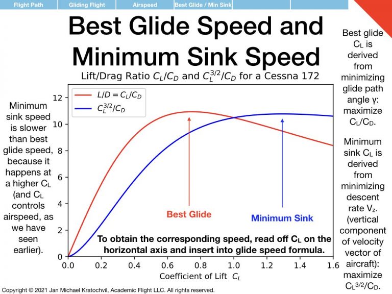
We see immediately from the glide path angle equation above that minimizing $\gamma$ (in the sense of making it as close to zero as possible) corresponds to minimizing $D/L$, which corresponds to maximizing $L/D$. The latter is what pilots are routinely taught in pilot training, that best glide distance happens at maximum $L/D$.

$C_L$ and $C_D$ Determine Glide Distance

The above equation for glide path angle $\gamma$, and therefore for glide distance, is extremely insightful and lets us immediately read off much of what the pilot must otherwise simply memorize about gliding flight. First of all, we notice that the righthand side does not depend on aircraft mass $m$ and air density $\rho$. So the glide path angle $\gamma$ and glide distance will be independent of aircraft weight and air density. In fact, the glide distance only depends on the coefficients of lift and drag, $C_L$ and $C_D$.

Remembering that the drag coefficient is given by
\begin{equation}
C_D = C_{D_0} + KC_L^2
\end{equation}
and the zero-lift drag coefficient $C_{D_0}$ and constant $K$ are both constants if we do not change the flap setting, we realize that coefficient of lift, $C_L$, alone determines glide path angle $\gamma$ and therefore glide distance. This is an extremely important realization. Apparently, there is one particular value of $C_L$, which will minimize our glide path angle and maximize our glide distance.

Best Glide Angle of Attack

For a given fixed flap setting (usually flaps retracted to maximize glide distance) $C_L$ only depends on angle of attack $\alpha$. For angles of attack $\alpha$ well below critical angle of attack $\alpha_c$, the lift curve is linear and the following relation holds
\begin{equation}
C_L = a(\alpha-\alpha_0)
\end{equation}
where $a=\partial C_L/\partial \alpha$ is the lift slope and $\alpha_0$ is the zero-lift angle of attack, i.e. the angle of attack at which the airfoil produces no lift.

Therefore, well below stall, the above equation is invertible and there is exactly one value of $\alpha$ corresponding to a particular value of $C_L$. Thus, if we have an angle of attack indicator in the aircraft, there can be a marking, typically marked by a blue dot, denoting the angle of attack which leads to the farthest glide distance in straight gliding flight in a power-off emergency. And this value of $\alpha$ is independent of airplane mass and air density. (This is much better than using a best glide speed as a reference, which, as we will see shortly, depends on airplane mass. We shall remember this for our airspeed discussion.)

If we do not have an angle of attack indicator in the aircraft, not all is lost. Since the best glide $\gamma$ and the best glide angle of attack $\alpha$ are both (each separately) the same, regardless of airplane mass), the corresponding pitch angle with the horizon, $\theta=\gamma+\alpha$, is always the same. Therefore, the nose of the aircraft should be below the horizon by exactly the same angle for any aircraft mass or air density to achieve best glide distance. (However, since every pilot has a slightly different viewing angle when sitting in the cockpit, each pilot would have to figure out this position on the windshield, where the horizon intersects it, themselves.)

Effect of Drag (and Flaps) on Glide Distance

Further, we realize from the above glide path angle equation that flap extension has a large effect on glide distance, because flaps increase drag $C_D$ (primarily by changing $C_{D_0}$ in the expression for the drag coefficient), and drag greatly affects the glide distance.

Glide Speed

Derivation of General Airspeed Equation of Gliding Flight

To obtain the glide speed from our two force equations
\begin{eqnarray}
D &=& – W \sin \gamma\\
L &=& W \cos \gamma.
\end{eqnarray}
we must first square them and add them together, resulting in the equation $L^2+D^2 = W^2 (\sin^2 \gamma+\cos^2 \gamma) = W^2$, where in the last step we have used the trigonometric identity $\sin^2 \gamma+\cos^2 \gamma=1$, which holds for any angle.

Using the equations defining the lift and drag coefficients as well as $W=mg$ yields
\begin{equation}
\frac{1}{2^2}\rho^2 V^4 S^2 (C_L^2+C_D^2) = m^2g^2
\end{equation}
which we can solve for airspeed $V$ yielding the airspeed equation in gliding flight:
\begin{equation}
V = \sqrt{\frac{2mg}{\rho S \sqrt{C_L^2+C_D^2}}} \approx \sqrt{\frac{2mg}{\rho S C_L}}.
\end{equation}
In the last step we have used the approximation $C_L^2>>C_D^2$, such that the drag coefficient can be neglected to a good degree of accuracy compared to the lift coefficient in the sum under the second square root. This is typically well satisfied, because lift is usually much larger than drag for reasonable airplane designs (if lift was equal to drag, we would get a $45^\circ$ glide path angle from the glide path angle equation, which would be extremely steep).

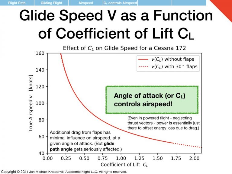
$C_L$ Determines Airspeed in Gliding Flight

From the above approximation we see that coefficient of lift $C_L$ determines airspeed $V$ in gliding flight, while the effect of drag on airspeed in gliding flight is negligible. This translates to angle of attack $\alpha$ determining airspeed in gliding flight, a fact particularly well known to glider pilots.

If this seems counterintuitive to the power pilot, who is used to drag opposing thrust from the engine in the straight-and-level flight picture, and to more engine power resulting in faster flight, consider the following. Yes, drag dissipates energy; but rather than taking the energy out of the kinetic energy of the aircraft and slowing it down, the airplane simply takes the energy out of the potential energy stored in its altitude and starts to sink faster, resulting in a steeper glide path at the same airspeed, if coefficient of lift $C_L$ is kept the same as drag $C_D$ is increased. This is consistent with our earlier observation that drag greatly influences glide path angle and therefore glide distance.

Best Glide Speed

We have noted earlier that best glide distance is achieved at a certain specific $C_L$. Via the above airspeed equation this results in an airspeed, the so called best glide speed, resulting in the largest glide distance from a given altitude.

Best Glide Speed Depends on Airplane Mass $m$

We note though that, unlike the glide path angle equation, the airspeed equation in gliding flight depends explicitly on on the aircraft mass $m$. Since best glide distance always occurs at the same $C_L$, naturally best glide speed will depend on aircraft mass, and this dependence goes as the square root of mass, $\sqrt{m}$. That is why the pilot’s operating handbook of the aircraft lists the best glide speed at maximum gross weight and oftentimes also at a few other weights. In case it is not published for other weights, the pilot can easily compute the best glide speed $V_{g}^{\mathrm{actual}}$ for their actual airplane weight from the published best glide speed at maximum gross weight, $V_{g}^{\mathrm{max\ gross}}$, by using the following formula, which follows immediately from the above airspeed equation for gliding flight, while remembering that $C_L$ is the same in both cases to get best glide path angle $\gamma$:
\begin{equation}
V_{g}^{\mathrm{actual}} = V_{g}^{\mathrm{max\ gross}} \sqrt{\frac{m_{\mathrm{actual}}}{m_{\mathrm{max\ gross}}}}
\end{equation}

Best glide speed also depends on air density $\rho$, but this is true only for true best glide speed $V$, not for indicated airspeed. Indicated airspeed essentially equals equivalent airspeed (neglecting position and instrument error as well as compressibility effects), and equivalent airspeed $V_e$ is independent of air density, having been defined as
\begin{equation}
V_e := \sqrt{\frac{\rho}{\rho_0}} V,
\end{equation}
where $\rho_0$ denotes the air density at sea level at on a standard day (standard atmosphere, i.e.\ at $15^\circ$C and $29.92$ in Hg).

Minimum Sink Speed

Concept of Minimum Sink Speed

Best glide coefficient of lift and best glide speed give the best glide distance. But they do not give the smallest sink rate, i.e. the maximum time aloft. It turns out that if the pilot wants to maximize the time in the air rather than the glide distance, a larger $C_L$ and a smaller airspeed must be chosen. Maximizing ones time aloft is useful if the pilot has already made the emergency landing site and is trying to maximize the time attempting an engine restart (or going through the shutdown procedure) or to communicate with ATC before getting below an altitude at which the transmission can be received.

Glider pilots also find this airspeed useful while termalling: they are trying to gain as much altitude as possible in the rising column of air, which is achieved if the inherent sink rate of the glider is minimized. Since they are flying circles, they are not going anywhere and do not care about covering any ground. On the contrary, a slower airspeed will allow them to make a tighter circle at a given bank angle, which may be advantageous to stay in the strong core of a tight thermal. Therefore, minimum sink speed is a well known concept to the glider pilot, but somehow it is omitted in standard power pilot education.

Flight Test Technique

The minimum sink speed is published in the glider pilot’s operating handbook. Yet most pilot’s operating handbooks for single engine airplanes do not list a minimum sink speed at all and do not even mention the concept. However, the pilot can determine minimum sink speed themselves experimentally quite easily, much more easily than it would be to determine best glide speed experimentally. Simply find out at which airspeed the aircraft shows the smallest sink rate on the vertical speed indicator (VSI), preferably on a calm day with not thermals, such as early in the morning. Also determine the airplane weight during the test flight, as this will let you scale the determined minimum sink speed value for different aircraft weights. Keep in mind that it if you do this with engine at idle instead of with engine shutdown and windmilling propeller, you will obtain a minimum sink speed which is larger than the actual in an engine failure situation (see our article on the effect of engine idle versus engine off on gliding flight).

Calculation of Minimum Sink Speed

We start with the same two force equations as for our previous calculations
\begin{eqnarray}
D &=& – W \sin \gamma\\
L &=& W \cos \gamma.
\end{eqnarray}
But this time we are not interested in the glide path angle $\gamma$, but rather in the sink rate $V_{z_{\mathcal{E}}}:=\dot z_E=V\sin\gamma$, which equals the vertical component of the airplane velocity vector $\mathbf{V}_{\mathcal{E}}=(V_{x_{\mathcal{E}}}, V_{y_{\mathcal{E}}}, V_{z_{\mathcal{E}}})$ in the inertial/world frame $\mathbf{E}$ (we are again assuming still air with no wind here). (Note that $V_{z_{E}}\not = w$, because the velocity components $\mathbf{V}_{\mathcal{B}}=(u,v,w)$, which we usually encounter, are in the body frame $\mathcal{B}$, while the sink rate is the velocity component along the vertical ($z_\mathcal{E}$-)axis of the inertial frame $\mathcal{E}$.)

Proposition (Sink Speed): The general sink speed equation in gliding flight is (approximately) given by
\begin{equation}
V_{z_\mathcal{E}}=\sqrt{\frac{2mg}{\rho S}} \frac{C_D}{C_L^{3/2}}
\end{equation}
and the minimum sink speed $V_{z_\mathcal{E}}$ is achieved at the value of $C_L$ which minimizes $C_D/C_L^{3/2}$.

Proof: From the first force equation above, $D = W \sin \gamma$, we can eliminate $\sin \gamma$ in the expression $V_{z_\mathcal{E}}=V\sin \gamma$. Then, using $W=mg$, $D=\frac{1}{2}\rho SV^2C_D$, and the general approximate glide speed formula $V\approx\sqrt{\frac{2mg}{\rho SC_L}}$ obtained earlier, we get:
\begin{equation}
V_{z_\mathcal{E}} = V \sin \gamma = V\frac{D}{W} = V \frac{\frac{1}{2}\rho SV^2C_D}{mg} = \frac{\frac{1}{2}\rho SV^3C_D}{mg} = \frac{\frac{1}{2}\rho S\sqrt{\frac{2mg}{\rho SC_L}}^3 C_D}{mg} = \frac{\sqrt{\frac{2mg}{\rho S}}}{C_L^{3/2}} C_D= \sqrt{\frac{2mg}{\rho S}}\frac{C_D}{C_L^{3/2}}.
\end{equation}
This expression holds generally for sink rate. Unlike the expression for glide angle $\gamma$ obtained earlier, $V_{z_\mathcal{E}}$ also depends on $m$ and $\rho$.

The $C_L$ that leads to $V_{z_\mathcal{E}}$ being the smallest possible, is the $C_L$ that minimizes $\frac{C_D}{C_L^{3/2}}$. This value of $C_L$ depends only on airplane design and does not depend on aircraft mass $m$ and $\rho$, even though the final sink rate $V_{z_\mathcal{E}}$ does, because the variables $m$ and $\rho$ do not occur in the expression for the drag coefficient $C_D=C_{D_0}+KC_L^2$ and therefore do not occur in the expression $\frac{C_D}{C_L^{3/2}}$, which is to be minimized.
q.e.d.

Glide Polar

The glide polar is a curve that plots the sink rate as a function of airspeed for a particular aircraft. It is often used by glider pilots not only to determine best glide and minimum sink speeds (which are usually also given numerically in the pilot’s operating handbook), but also to adjust best glide speed for headwind and tailwind. A useful rule of thumb to maximize your glide distance is to add half the wind speed to your best glide speed, if flying into a headwind, because you want to get to your destination faster, giving the headwind less time to blow you backwards. On the other hand, in the presence of a tailwind, you would want to fly slower (at a slower sink rate) giving the wind more time to push you from behind. The rule of thumb here is to subtract half the tailwind speed from your best glide speed, but you should never fly slower than minimum sink speed, because that would only increase your sink rate (and reduce your time aloft), while making less forward progress.

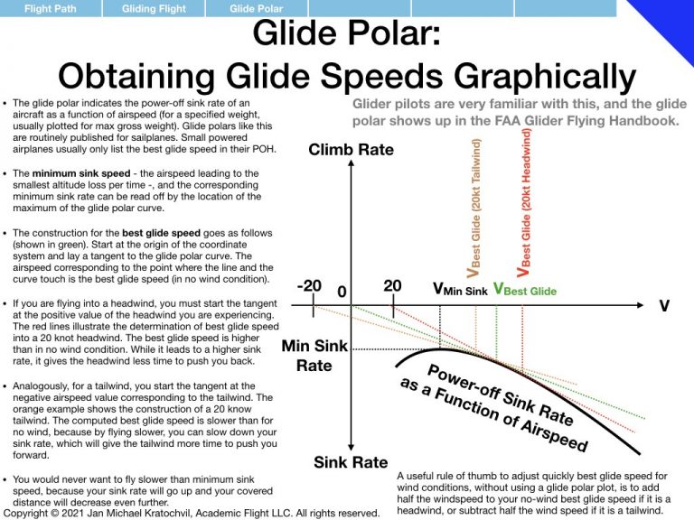
However, there is a more accurate way to determine these glide speed adjustments for headwind and tailwind, using the glide polar. The figure on the right, taken from the slides of our flight dynamics ground school, illustrates the construction and determination of these adjustments.

Aircraft Control in Straight Gliding Flight

Use of Flaps During Gliding Flight

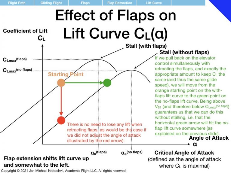
Flaps resemble in some sense a negative throttle in that they create drag, which can be interpreted as negative thrust. But they also create more lift and their use therefore is a little more involved. We would therefore like to start our discussion of aircraft control with a cautionary note on flap retraction during gliding flight, and why one actually does not have to worry about the loss of lift if proper understanding is present and appropriate, simultaneous, compensating control inputs are performed.

We have observed previously that the coefficient of lift determines glide speed and that the coefficient of drag is negligible. This means that flaps have no effect on glide speed, provided the pilot keeps the coefficient of lift the same. This requires a reduction of angle of attack by the pilot if camber is increased due to flap extension to maintain glide speed. Conversely, if flaps are retracted, the pilot can compensate for the loss of lift due to flap retraction by increasing the angle of attack, provided the airplane is flying at an airspeed of $V_{S1}$ or larger (stall speed with flaps retracted). Flap retraction leads only to inevitable loss of lift/altitude or stall, if the airspeed is below $V_{S1}$. If the airplane is trying to make a power-off emergency landing, the pilot should be flying close to best glide angle of attack, resulting in a best glide speed well above $V_{S1}$. Therefore, flaps can be extended and retracted at will, without immediate loss of lift/altitude, if the pilot compensates appropriately with the elevator control simultaneously.

So what do flaps do? If airspeed is kept the same, this means that coefficient of lift is kept the same. So a change in flap setting only changes the coefficient of drag. We see from the glide path angle equation that the coefficient of drag has a dramatic effect on glide path angle. Flaps therefore control the glide path angle, not the airspeed. (However, as we shall see, a crucial element in this reasoning is the assumption that $C_L$ is kept the same by a corresponding simultaneous adjustment of the elevator control.)

Control Parameters and Functional Dependencies of Aerodynamic Parameters

It is important to realize that actual aircraft control by the pilot may not necessarily follow the physical relations above. In the above calculations, we have often spoken about $C_L$ and $C_D$ as the control parameters, but those are not the ones the pilot has direct control over, and furthermore, it is even difficult for the pilot to determine their value. Furthermore, as we have seen, they are not even independent, as $C_D$ depends on $C_L$ via $C_D=C_{D_0}+KC_L^2$.

The independent, direct control parameters available to the pilot are the elevator deflection $\delta_e$ and the flap setting $\delta_f$ (or the spoiler setting in the case of a glider or airplane with spoilers or dive brakes). $\delta_e$ affects the pitching moment and thereby lets the pilot select the angle of attack $\alpha$ (taking into account longitudinal stability considerations). This translates into a selection of $C_L$, but $C_L$ also depends on the flap setting $\delta_f$. The drag coefficient also depends on $\alpha$ (via $C_L$) and $\delta_f$. Thus we can write for the functional dependencies
\begin{eqnarray}
C_L&=&f(\delta_e, \delta_f)\\
C_D&=&g(\delta_e, \delta_f)
\end{eqnarray}
for some functions $f$ and $g$. This couples both controls to both parameters, and the separation we sought earlier on physical grounds is not actually what is controlled by the pilot.

While both controls control both variables, which is why they should therefore be used in a coordinated fashion, procedurally it is nonetheless useful to seek some mental separation, because this gives the pilot a procedural prescription how to respond to a perceived deviation in glide path (altitude) and/or airspeed.

Final Approach Control Techniques

The two techniques discussed in this section are applicable only on final approach, when both flight path and airspeed are to be controlled precisely. Before that, i.e. anytime before the base-to-final turn, airspeed is to be controlled with angle of attack (i.e. elevator control $\delta_e$). The flaps should remain retracted (a slip may be performed to dissipate excess altitude). If the airplane is super high, the pilot is to circle over the landing area to take a good look at the emergency landing sight. Ideally a small airplane would be positioned at 2000 ft AGL in direction of flight over the intended touchdown point and at 1000 ft AGL on the downwind leg abeam the touchdown point. Once the base-to-final turn is performed (or if a longer straight-in approach is executed), then the pilot may choose between one of these two techniques (they both have their merit and drawbacks).

Technique 1: Elevator controls Airspeed and Flaps control Glide Path Angle

The most natural and classic assignment based on the physical reasoning above is to associate the elevator with airspeed control and the flaps (or a sideslip) with glide path (and thus altitude) control. This is often done successfully, however, it is not the only way and while it is the most physical way, it is not the most humanly intuitive way. It is also not the most efficient way in terms of static control stability: if the aircraft is too high and too fast, pulling on the elevator will not only slow it down, it will also make it climb more, and this (at least initially) deviate more from the flight path.

Technique 2: Elevator controls Glide Path and Flaps control Airspeed

It is possible to assign the elevator to glide path control and the flaps to airspeed control. This technique uses the natural sense of the pilot’s brain for direction: it is much easier for the pilot to pitch for the runway with the elevator than to infer what flap setting is needed to maintain glide path. With this technique, the flaps are then extended or retracted depending on airspeed (the elevator must be adjusted simultaneously to compensate for the change of coefficient of lift during a change in flap setting). We have discussed above that flap retraction does not lead to a loss of lift that the pilot cannot compensate for, as long as the airplane flies above stall speed with flaps retracted, $V_{S1}$. For best glide speed, this is obviously the case, and in fact, during this approach the pilot will want to approach at an airspeed noticeably higher than best glide speed, because if the airplane gets too low and the pilot pulls back on the elevator to get back on glide path, one would want any associated decrease in airspeed to bring the airplane closer to best glide speed and thus to assist in the return to the glide path further, rather than dropping below best glide speed and in the long run to lead to an even shorter glide distance.

One distinct advantage of this method is that any responses to deviations from the desired condition lead to improvement, i.e. there is no situation where the aircraft’s initial response would actually get you farther away in one of the variables of airspeed or glide path, as was the case in the first method we introduced.

This second technique of glide path and airspeed control is used, for instance, by glider pilots in the steep landing approach (as opposed to the regular landing approach). In the steep approach, the glider pilot comes in seemingly insanely high, in a fashion that one would a priori not believe that it would still be possible to land the glider on the runway without overshooting. Then the pilot deploys full spoilers and simply dives for the runway using the elevator. While this does not work in every glider make and model, many will essentially reach a terminal dive velocity with spoilers extended which is still within their operating limits. If the airspeed eventually starts to drop as the glider aims for the runway in this fashion, the spoilers can be retracted a bit, keeping the speed still relatively high, well above best glide speed and at a glide path angle well above normal. Any excess airspeed is bled off with full spoiler deployment shortly before roundout (or the spoilers can be carried into the roundout if necessary).

In this approach, clearly, elevator controls glide path and spoilers control airspeed in the mind of the pilot. The benefit of this approach is that there is an abundance of potential and kinetic energy at any given point – much more than during the traditional approach – and the odds of getting into an unexpected strong sink on final approach and coming up short of the intended landing site is essentially eliminated.

This technique can be adopted by the power pilot in an engine-out situation as well, albeit with much less airspeed control using flaps (which is why the approach cannot be started insanely high). The challenge lies in keeping the airspeed (well) above best glide speed until on short final, where it is bled off with full flap deployment, yet at the same time keeping the airspeed within the white arc (allowed airspeed region for flaps extended). But the principles are the same.