On this page we give a concise introductory overview of some of the main topics involving autonomous flight and vehicle autonomy in general. They are grouped into four chapters:
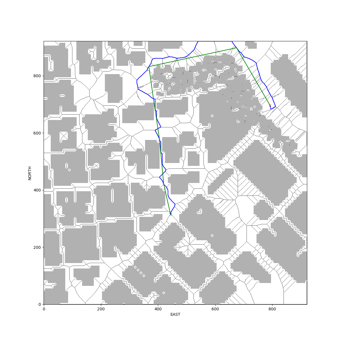
- Path Planning
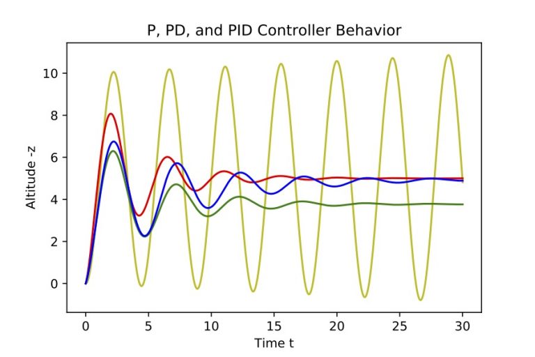
- Vehicle Control
- Vehicle State Estimation (position, velocity, attitude, etc., from onboard sensors)
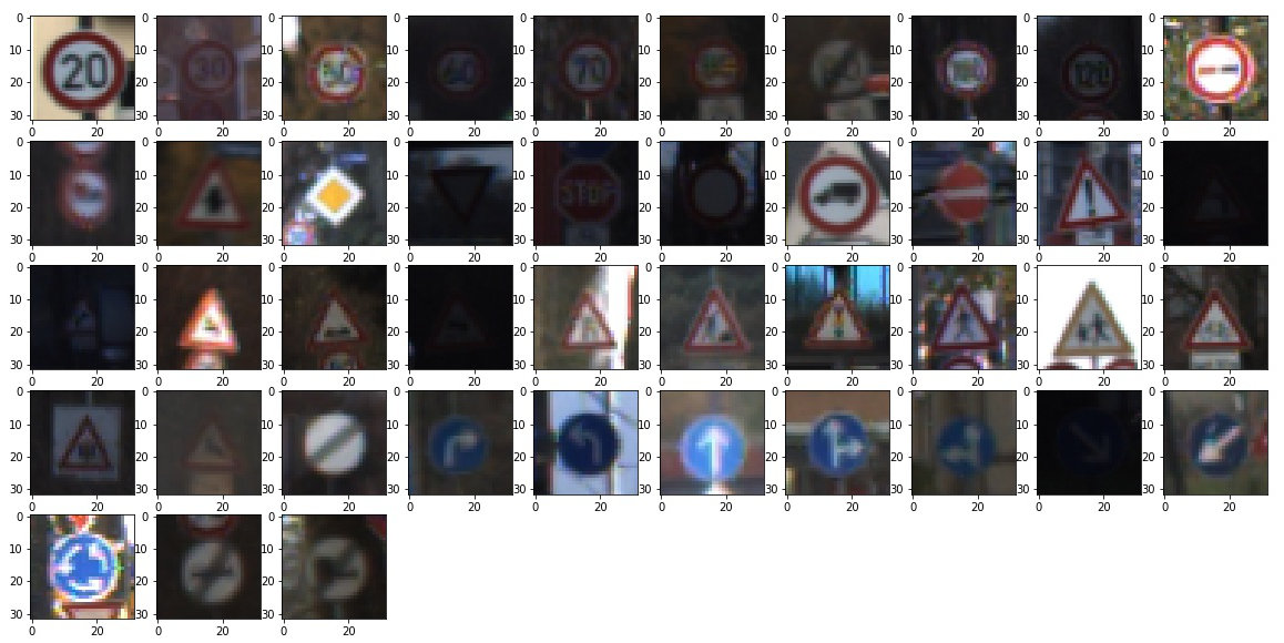
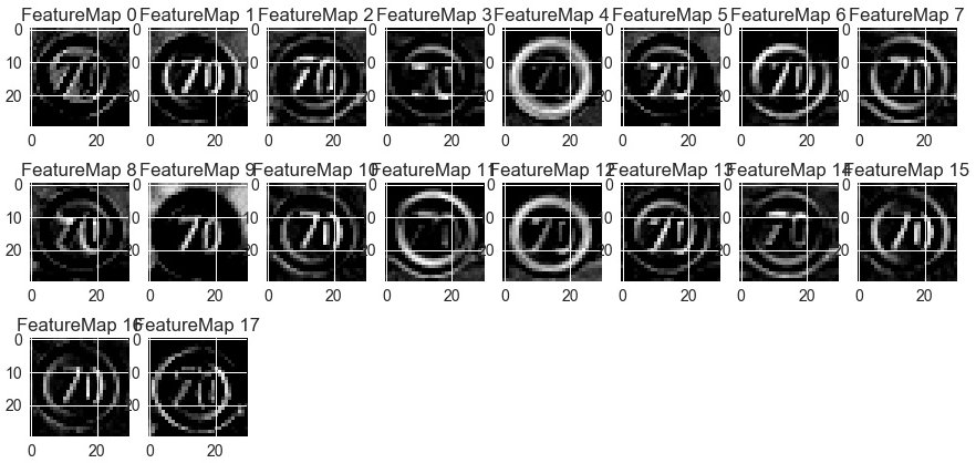
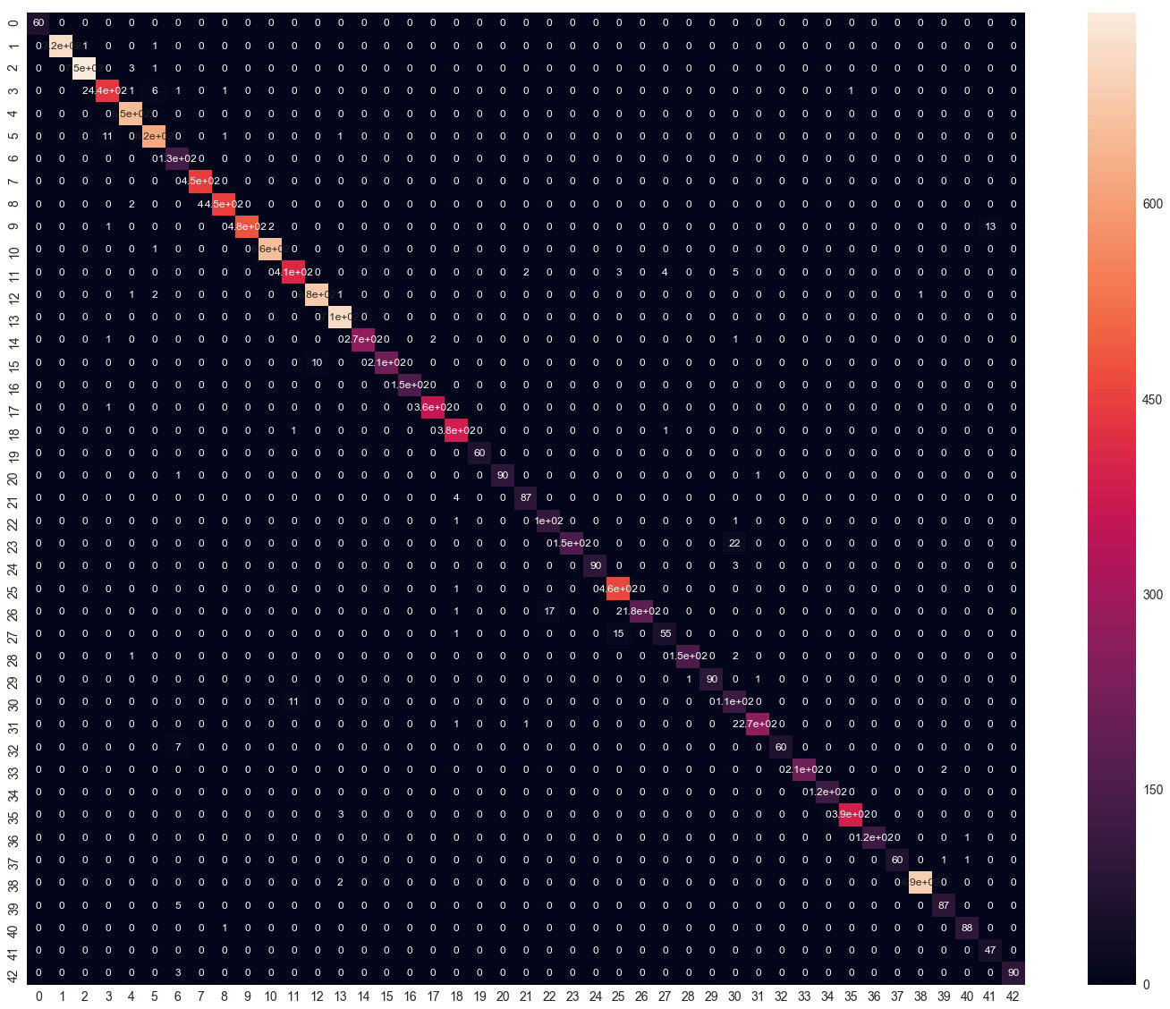
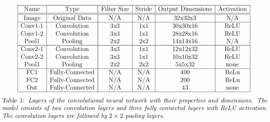
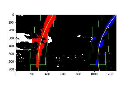
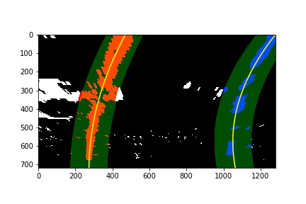
- Computer Vision
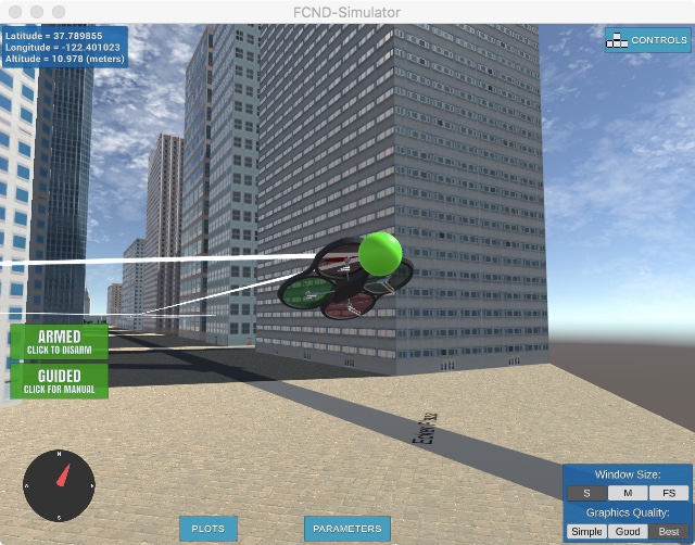
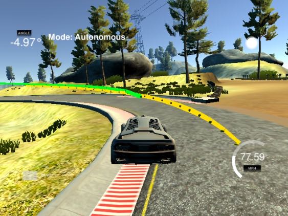
Many of the examples below, especially the visual presentations of the simulations, originate from Udacity’s Flying Car and Autonomous Flight Engineer Nanodegree and the Self-Driving Car Engineer Nanodegree programs. We encourage you to take a look at these programs on the Udacity website.
We currently offer short courses in vehicle state estimation and vehicle control, which are somewhat complementary in nature. They dive deeper into selected topics than, for instance, the above Nanodegrees, but without the spectacular visuals and without offering the broad overview of vehicle autonomy that the above programs provide. They are also much heavier on the mathematics, including derivations and not just application of formulas. They are suitable either for people who have a need for only a single topic in more detail (e.g. attitude estimation from iPhone IMU data), or who have taken courses similar to the above and want to improve their understanding of certain aspects.
The prerequisites for all our autonomous flight courses are a solid familiarity with Python (including classes), and basic familiarity with undergraduate-level linear algebra (vector spaces, matrices, matrix inversion, etc.) and multivariable calculus (total and partial derivatives, integrals, etc.). If you lack some of these prerequisites, we can help you obtain them. There are also plenty of introductory math and programming courses available on online learning platforms like Coursera, many of which you can audit for free.