PPGS 2023-2024, Lecture 2: 2D and 3D Aerodynamics – Selected Presentation Slides
Preamble: A First Look at the Atmosphere
Before we get into aerodynamics, let us make a brief statement about the atmosphere. We will discuss the atmosphere in more detail later (including the International Standard Atmosphere (ISA)), but for now let us just state that the atmosphere is a gas. As such, it can be described by the thermodynamic quantities:
- Pressure: \(p\) [in Hg] – for ambient pressure, pilots use pressure altitude, which has units [ft]]
- Temperature: \(T\) [˚C]
- Density: \(\rho\) [kg/m3, slugs/ft3] – pilot use density altitude, which has units [ft]
The units above are those typically used by pilots and reported to them by aviation weather services. We will discuss them later.
Being a gas, the air obeys (approximately) the ideal gas law:
\begin{equation}
p = R \rho T
\end{equation}
where \(R\) is the specific gas constant for air. The ideal gas law relates pressure to density and temperature. If we know two of these three quantities, it lets us compute the third.
As a side note before moving on, note that the above equation expects the temperature T to be given on an absolute temperature scale, i.e. in Kelvin [K] (the absolute temperature scale related to Celsius) or in Rankin [R] (the absolute temperature scale related to Fahrenheit), depending on what units the specific gas constant \(R\) is provided in.
Aircraft Performance and Atmospheric Measurements
Aircraft performance (such as climb angle and rate, takeoff and landing distance) depends on air density \(\rho\). This is a very important piece of information every pilot must keenly be aware of, so let us repeat it: aircraft performance depends on air density.
As luck would have it, of course, there is no simple device to carry with us on an airplane, which would measure air density directly. Instead, we are forced to measure temperature (with a thermometer) and pressure (with the altimeter, which is really just a barometer with a funny altitude scale), and then compute the air density with the ideal gas law. From this air density, we can then determine aircraft performance. (The funny altitude scale of the altimeter leads to the concepts of pressure altitude and density altitude, which are concepts we will discuss some other time). In today’s lecture we just want to focus on the physics concepts, not on measurement units.
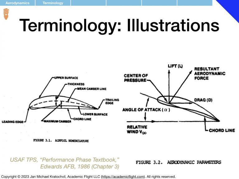
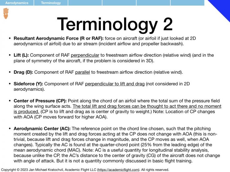
The Resultant Aerodynamic Force on an Object in an Airflow
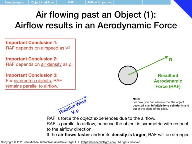
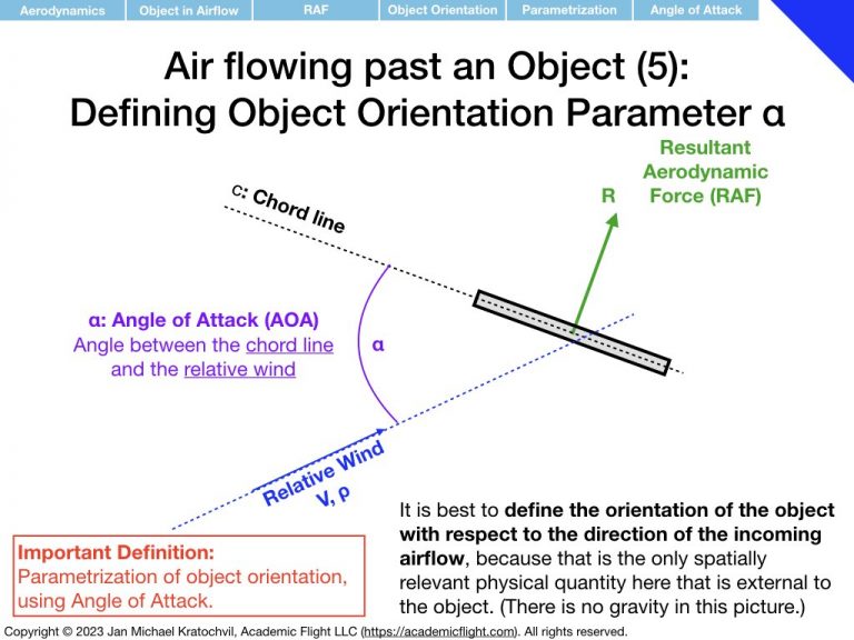
In the set of slides below we study the Resultant Aerodynamic Force (RAF) that an object experiences when placed in an airflow, or – equivalently – when the object itself is moving against non-moving, still air, and thus experiencing a relative wind.
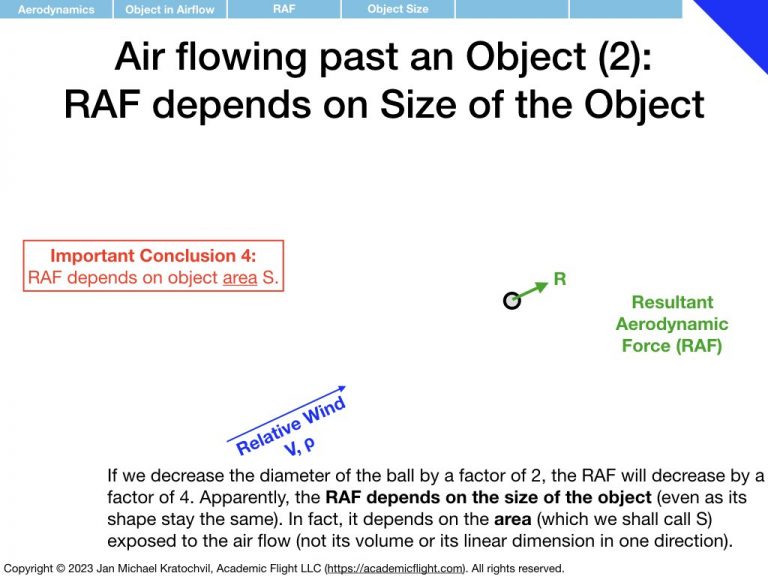
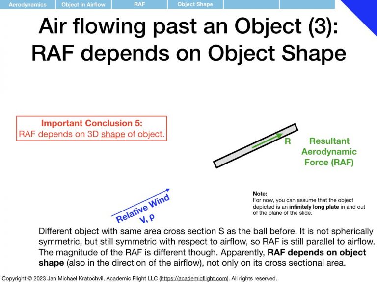
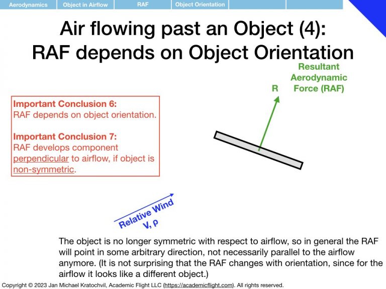
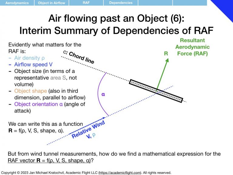
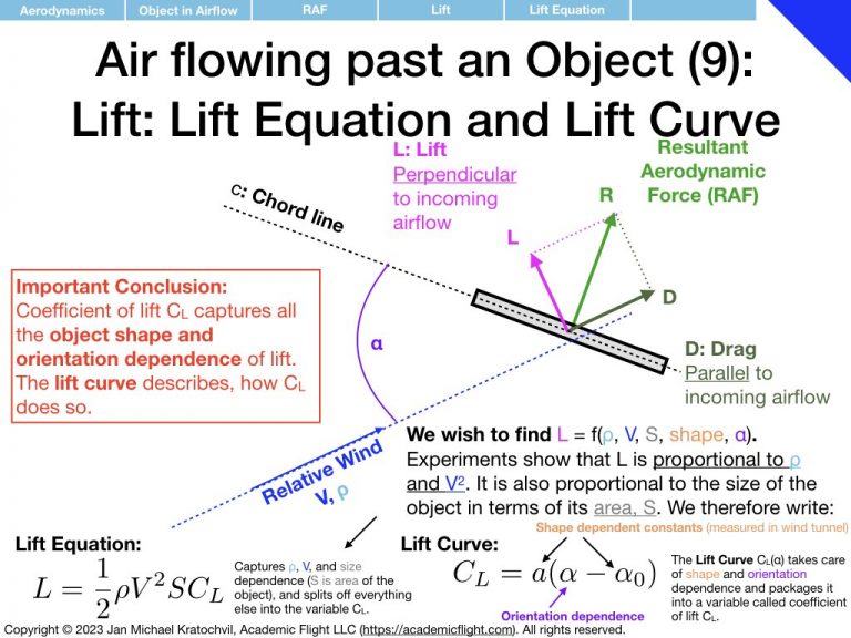
First we notice that the RAF is proportional to airspeed squared, V2, and to air density ρ. Then we realize that the RAF depends on the object area (think cross section exposed to the airflow – as opposed to its volume or just size measured in one dimension), which we shall label S. We proceed to find that object shape and orientation also matter. We parametrize object orientation by introducing the angle of attack α, as an easy way to keep track of orientation with a single number. Then we notice something remarkable: if the object is not symmetric with respect to the airflow direction, the RAF does not exclusively point in the same direction as the airflow, but rather also develops a perpendicular component.
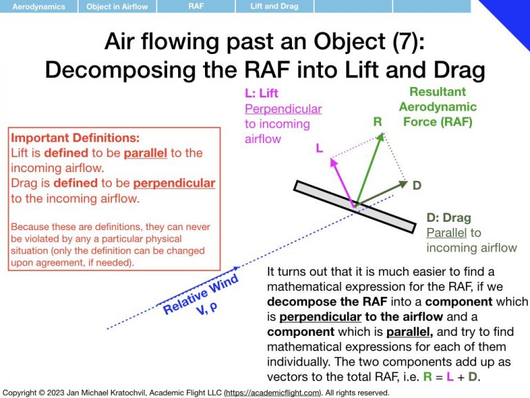
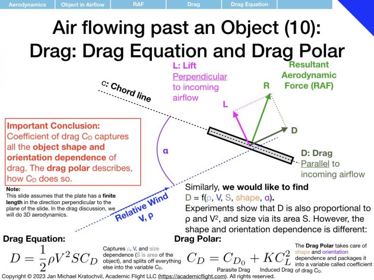
We decide to keep track of the perpendicular component separately from the parallel component, call the perpendicular component lift, and denote it by L. The component of the RAF parallel to the airflow direction shall be called drag and denoted by D. We note that this is a definition and can thus never be violated (unless we change the definition): lift will always remain perpendicular to the incoming airflow, and always orthogonal to drag, because that is how we defined the two components. In reality, they are both part of the RAF and an orthogonal decomposition thereof (in 3D, we will later also encounter sideforce, Y, which will be defined as being perpendicular to lift and drag, pointing in the third spatial dimension).
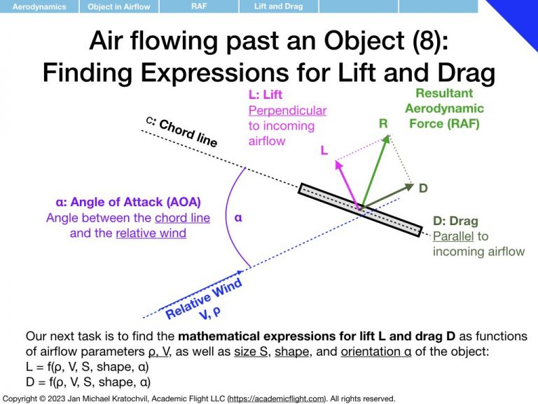
We then tackle the task of finding mathematical expressions for lift and drag as functions of the parameters they depend on, i.e. expressions for
\begin{eqnarray}
L &=& f(\rho, V, S, shape, \alpha)\\
D &=& f(\rho, V, S, shape, \alpha)
\end{eqnarray}
where parameter \(\alpha\), the angle of attack, captures the orientation of the object, and “shape” is still something we need to figure out how to deal with.
As a starting point, we write down the following mathematical expression, based on the dependencies we just observed (never mind the prefactor of 1/2):
\begin{eqnarray}
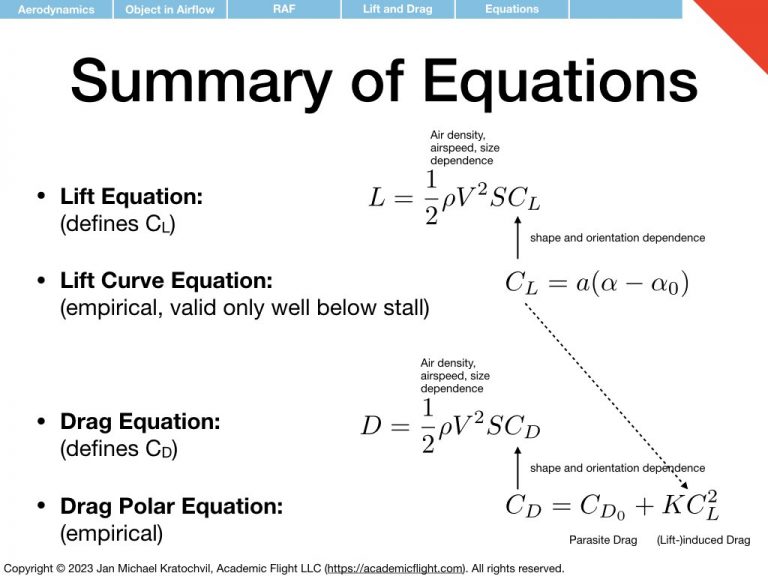
L &=& \frac{1}{2}\rho V^2 S C_L\\
D &=& \frac{1}{2}\rho V^2 S C_D\\
\end{eqnarray}
In this expression, we have dumped all dependence on shape and orientation of the object into the quantities \(C_L\) and \(C_D\), which we shall call coefficients of lift and drag. The dependence of lift and drag on air density, airspeed, and general size of the object are captured by the front part of the formulas. What remains to be determined is how \(C_L\) and \(C_D\) depend on object shape and orientation.
Orientation and Shape Dependence Encoded in CL and CD
Our goal is now to find a mathematical expressions for \(C_L\) and \(C_D\). They should be as simple as possible mathematically (simple expressions with few parameters), while still capturing the physics reasonable accurately. And they do not have to work for arbitrary object shapes: we will only be studying wings of aircraft, so we only need these expression to work for airfoil like shapes. The simple plate in the above slides is a good starting point, and similar shapes like this, which are designed to produce lots of lift and comparably little drag, when placed in an airflow, so that they are useful for building wings of aircraft.
Experimental evidence suggests that the following expressions are often good approximations of \(C_L\) and \(C_D\) for our purposes:
\begin{eqnarray}
C_L &\approx& a (\alpha-\alpha_0)\\
C_D &\approx& C_{D_0} + K C_L^2\\
\end{eqnarray}
where \(a\) is the lift slope, \(\alpha_0\) is the zero-lift angle of attack (often also written as \(\alpha_{L=0}\)), \(C_{D_0}\) is the parasite drag, and \(K\) is the induced drag prefactor. They are all parameters related to the exact shape of the object/airfoil, and their exact values need to be inferred from experimental measurements on that particular airfoil.
Again, the above expressions for \(C_L\) and \(C_D\) are just approximations (for instance, the expression for $C_L$ could be regarded as the first two terms of a Taylor series expansion, with any terms proportional to \(\alpha^2\) neglected). In particular, we will see that the approximation for \(C_L\) chosen above breaks down for high angles of attack, where the aerodynamic phenomenon of stall occurs, which has to do with airflow separation from the upper surface of the airfoil. We will discuss this shortly, when we talk about the fluid dynamics aspects of 2D aerodynamics in more detail.
Parametrizations of \(C_L\) and \(C_D\)
Why did we chose the above forms for \(C_L\) and \(C_D\), if they are just approximations? The answer is that the real \(C_L\) and \(C_D\) have a much more complicated dependence on angle of attack, but the extra complications do not change the result much. The above expressions fit experiments reasonably well, and we have managed to reduce this complicate problem to just four parameters: \(a\), \(\alpha_0\), \(C_{D_0}\), and \(K\). For any given airfoil, we can experimentally determine the values for these four numbers, and this will give us a sufficiently good approximation, while being easy to keep track off. More importantly, these simple expressions let us study the general effects of the airfoils on flight dynamics in an analytic, closed form fashion and gain valuable insights, which would otherwise perhaps be masked in a fully numerical approach.
Lift Curve \(C_L(\alpha)\) and Drag Polar \(C_D(C_L)\)
What we need to do next is to develop some intuition, what those expressions for \(C_L\) and \(C_D\) mean for the pilot. This is best done by studying the graphs of \(C_L\) and \(C_D\) as functions of angle of attack \(\alpha\) in the following two slides. They are called the lift curve and the drag polar, respectively. To develop intuition for the problem as pilots, we care more about these graphs than their underlying mathematical expressions, and, indeed, you will find these graphs in the PHAK in Figure 5-4.
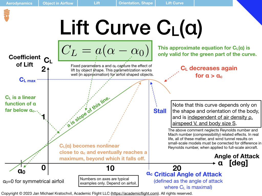
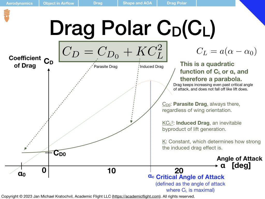
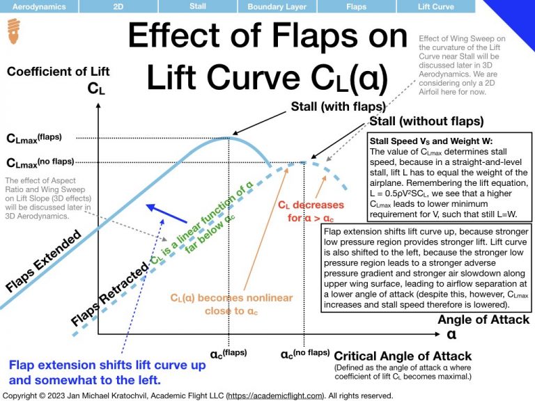
The most important thing to remember about the lift curve (left slide) is that after a linear rise the lift curve eventually peaks as some maximum \(C_L\) value – at an angle of attack which we shall call critical angle of attack, \(\alpha_c\). If we increase the angle of attack any further, we again get a smaller value of \(C_L\), which is undesirable. In addition, as we will study airflow properties later, flying at angles of attack beyond the critical angle of attack often leads to serious control difficulties of the aircraft and can lead to total loss of control, potentially resulting on a very serious accident.
As far as the drag polar is concerned (right slide), we notice that the coefficient of drag \(C_D\) increases quadratically with angle of attack \(\alpha\), and continues to increase even beyond the critical angle of attack \(\alpha_c\), steadily rising, even as the lift coefficient \(C_L\) starts to decay. This will have important ramifications later. The drag polar has two components: a component independent of lift coefficient, called parasite drag, and a component proportional to \(C_L^2\) responsible for the quadratic rise, called the induced drag.
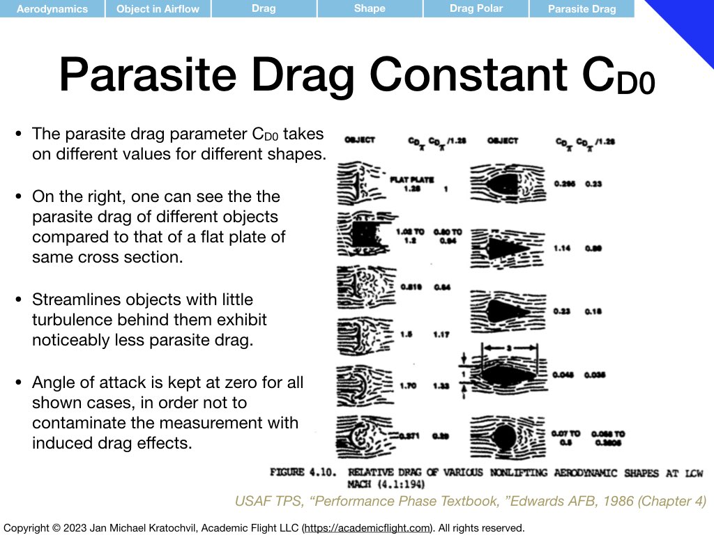
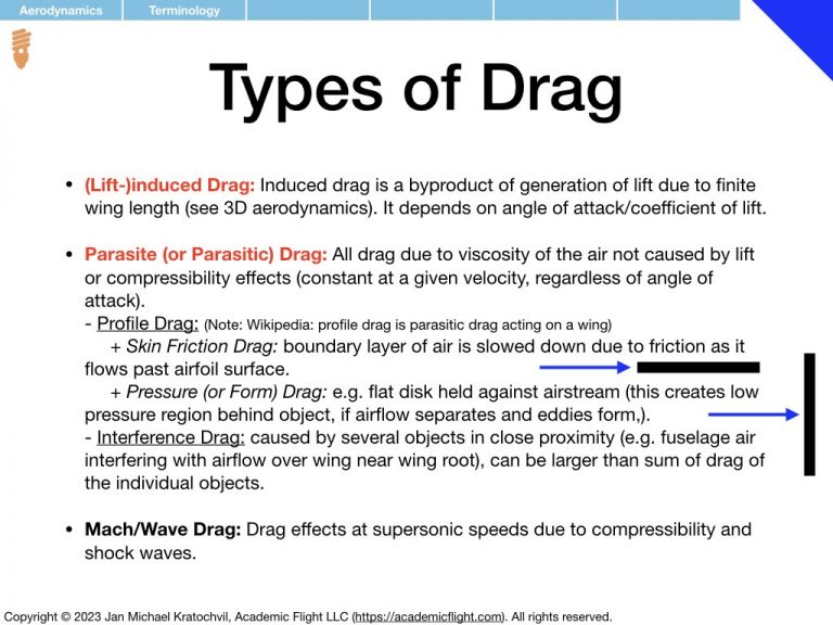
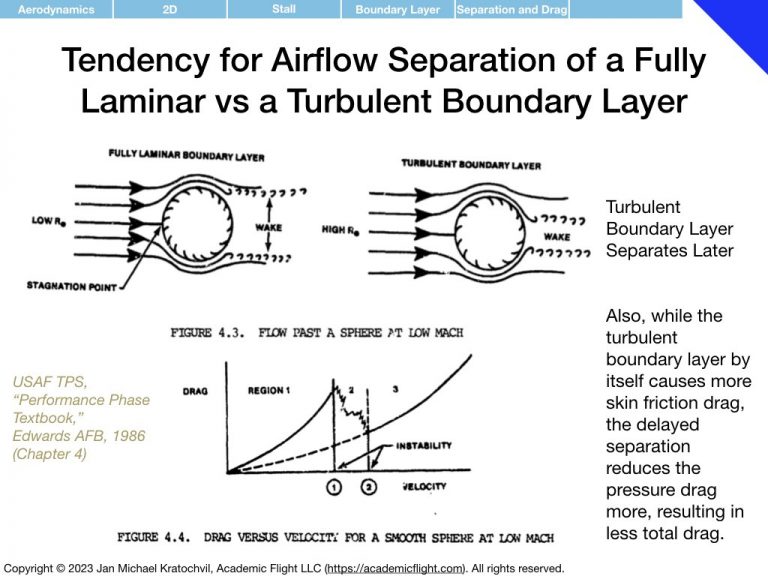
Parasite drag, \(C_{D_0}\), is the part of the drag that exists even when no lift is generated. It comes from two sources: profile drag and interference drag. Profile drag itself has two contributions: skin friction drag, originating from the airflow rubbing against the surface of the object as it flows by, and pressure (or form) drag, which comes from the pressure difference in front and behind the object due to airflow separation.
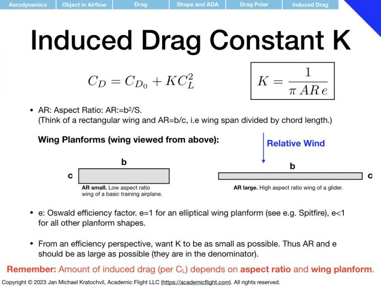
Induced drag, \(C_{D_i}=KC_L^2\), – induced by lift – is an unavoidable byproduct of lift generation by a wing of finite length (3D aerodynamic effect), and is related to the vortices forming at the wingtips (see later). For now we shall merely note that the induced drag parameter \(K\) depends on the aspect ratio of the wing, i.e. on the relation of the length of the wing span to the wing cord. The slide below illustrates this.
First Operational Conclusions for the Pilot
Now that we understand the general effect of airflow velocity, air density, size, shape, and orientation of an airfoil-like object (which is our case so far still has just been a flat plate), let us see if we can draw some first operational conclusions for the pilot, before we even dive into the finer points of aerodynamics. The right slide below draws these conclusions, and the left slide shows, where they come from in the equations we have just worked out.
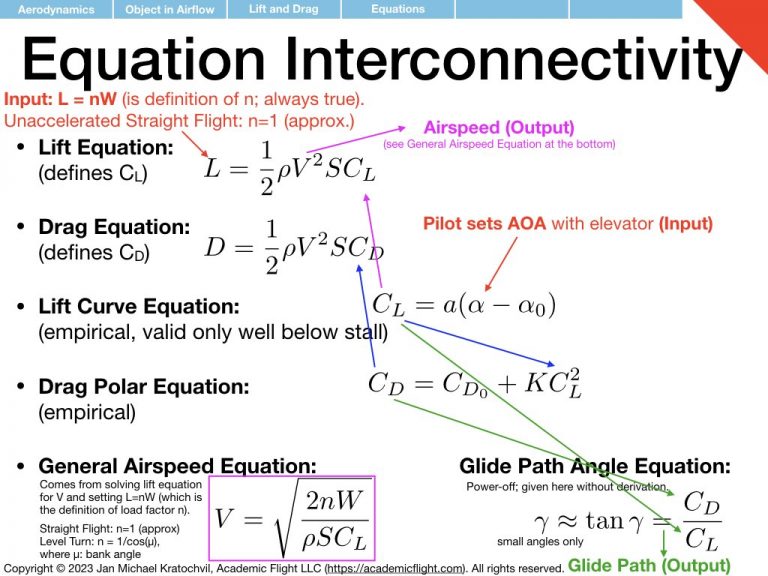
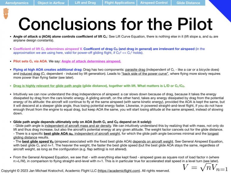
If it is confusing for you, how we arrived at the conclusions on the right-hand side from the equations on the left-hand side, you can either just memorize the conclusions (we added comments to assist in developing intuition), or you can scroll to the bottom of this page, where we provide an equation flowchart that lets you draw these conclusions on your own.
We do need to get deeper into aerodynamics though. While it looks like we can almost fly already, we have swept one important thing of 2D aerodynamics under the carpet in our equations: the nonlinear part of the lift curve associated with the aerodynamic stall. In what follows, almost everything is to build up the knowledge to understand this phenomenon and how the pilot can control it.
What we also need to cover in more detail is the aerodynamic origin of the induced drag factor \(K\). This we will do in the next lecture (Lecture 3), where we cover 3D aerodynamics. It has to do with the wingtip vortices of wings of finite length, and will lead us not only to a discussion of induced drag, but also to wake turbulence (and the associated hazards for other aircraft) and ground effect.
2D Aerodynamics: The Lift Curve
With some of the heavy conceptual lifting already out of the way, taken care of in the previous section, we venture to explain the shape of the lift curve from aerodynamics. In the process, will encounter a phenomenon called aerodynamic stall.
In short, let us first introduce Bernoulli’s principle, which states that the faster air flows, the lower its static pressure will be. Bernoulli’s principle states that the sum of static pressure \(p\) and dynamic pressure \(\overline{q}\) remains constant throughout the airflow, even as the air flows around the airfoil:
\begin{equation}
p + \overline{q} = \mathrm{const.},
\end{equation}
where \(\overline{q}:=\frac{1}{2}\rho V^2\) defines the dynamic pressure (dynamic pressure is pressure arising from the velocity of the airflow). One easily sees that if we increase dynamic pressure (due to an increase in airflow velocity \(V\)), static pressure \(p\) has to decrease, for Bernoulli’s equation to remain satisfied. (Note that when we simply say “pressure” below, we always mean static pressure; dynamic pressure will always be referred to explicitly as “dynamic pressure”.)
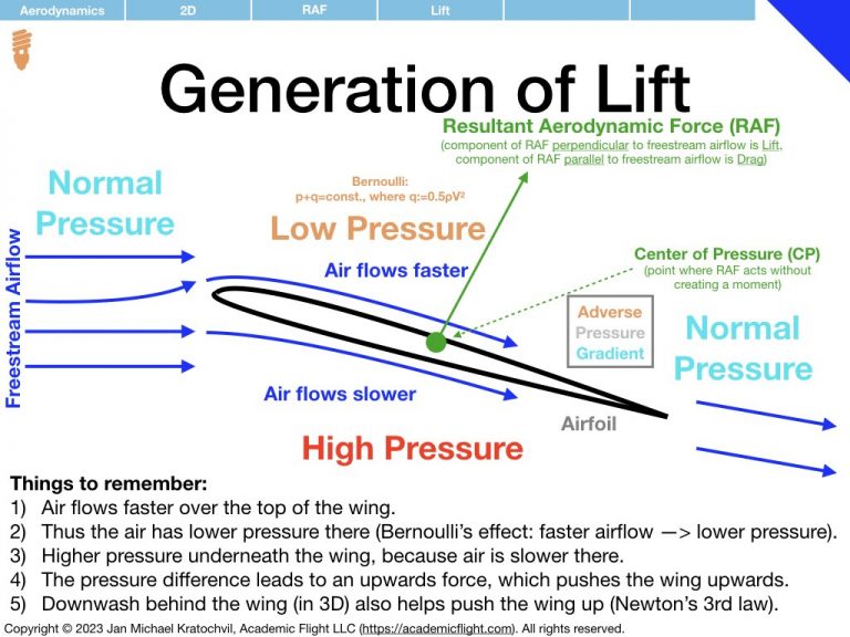
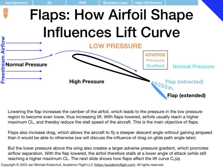
Due to the shape of the airfoil, the airflow above the wing flows faster than the freestream velocity of the undisturbed incoming air ahead of the wing, while the airflow below the wing is slowed down. By Bernoulli’s principle, this gives rise to a low pressure region above the airfoil and a high pressure region below the airfoil. This pressure difference leads to the lift force, which pushes the wing up (in 3D downwash behind the wing also contributes to the upward force, due to Newton’s third law of motion).
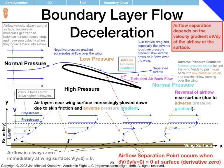
Meanwhile, normal pressure regions continue to exist of front of the wing and behind the wing. Thus the air above the wing travels from a normal pressure region to a low pressure region and then to another normal pressure region. Air likes to flow from higher pressure to lower pressure, so going from the normal pressure region ahead of the wing to the low pressure region above the wing accelerates the airflow (the creation of the low pressure region due to the accelerated airflow (Bernoulli) and the acceleration due to the pressure difference go hand in hand, one cannot say that one causes the other) . Similarly, going from the low pressure region to the normal pressure region behind the wing is something the air does not actually like to do: here the air must fight an adverse pressure gradient at the rear end of the airfoil.
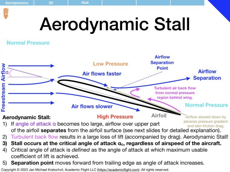
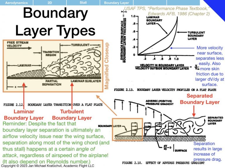
Fighting the adverse pressure gradient in the rear part of the airfoil slows the airflow down. The airflow may have been slowed down somewhat earlier already, due to rubbing against the upper wing surface, which is called skin friction drag. When the angle of attack is higher than the critical angle of attack, the weakened airflow does not have enough kinetic energy (speed) near the wing surface to make it to the trailing edge of the wing against the adverse pressure gradient, and – near the wing surface – air rushes in from the back, causing the airflow coming from the front of the wing to separate from the wing surface. This makes the airflow de facto see a different wing shape, and a lot of lift is lost. This is called an aerodynamic stall (usually referred to as stall for short). Furthermore, the turbulence caused by the air rushing in from behind causes lots of drag and prevents the control surfaces (ailerons) to work properly, which can lead to complete aileron ineffectiveness and loss of lateral control of the aircraft (which can lead to loss of directional control and the onset of an autorotation in both yaw and roll, in a phenomenon called a spin – we will see this later).
Even though we have explained the airflow separation from the upper surface of the wing, leading to a stall, by means of the airflow running out of kinetic energy and therefore speed, we want to emphasize that stall has nothing to do with airspeed of the aircraft. The stall is only dependent on angle of attack \(\alpha\). An airplane can stall at any airspeed, even much higher ones; what matters for stall is that the critical angle of attack is exceeded by the wing. Pilots must remember this very important fact.
Basic 2D Aerodynamic Concepts in Aerospace Engineering
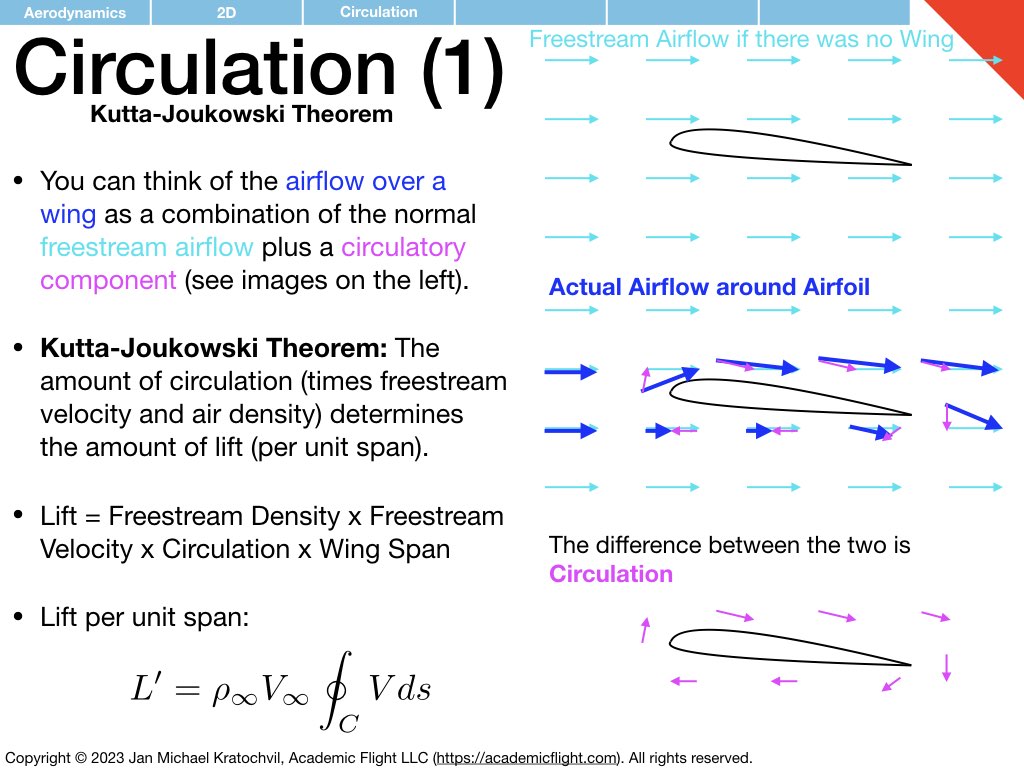
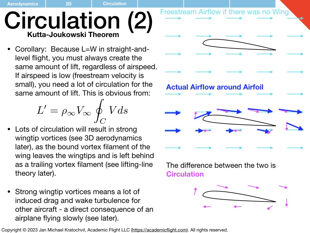
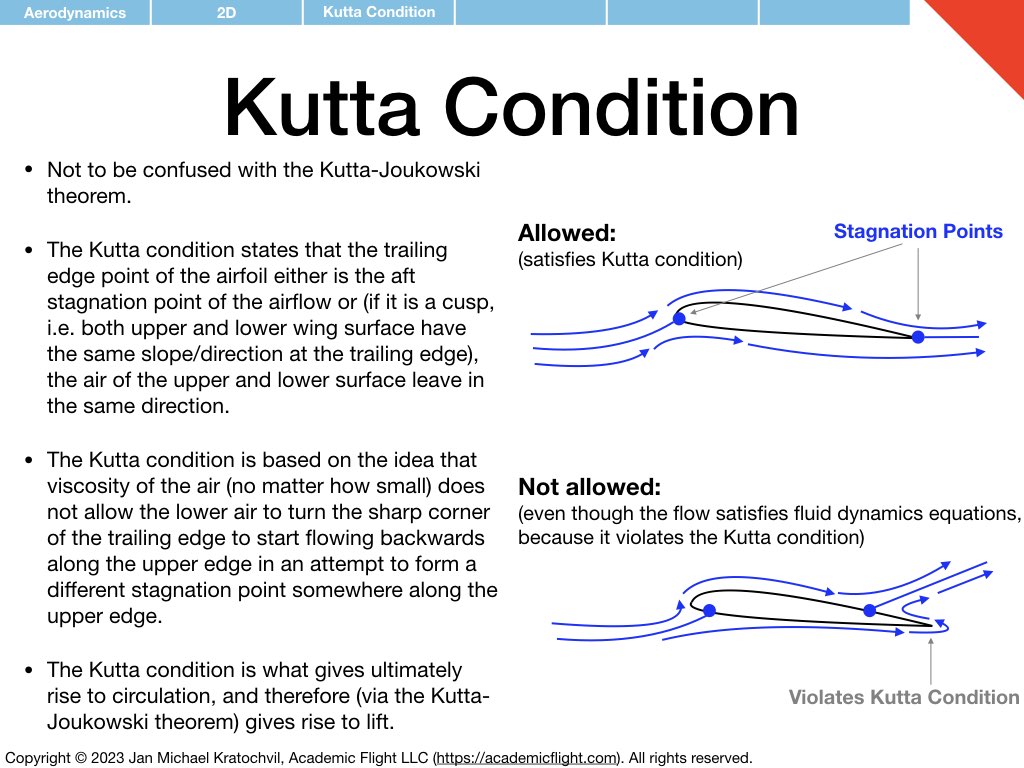
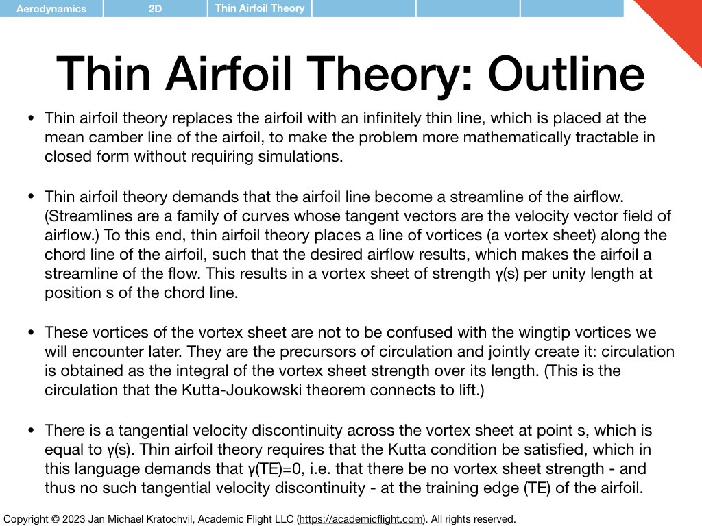
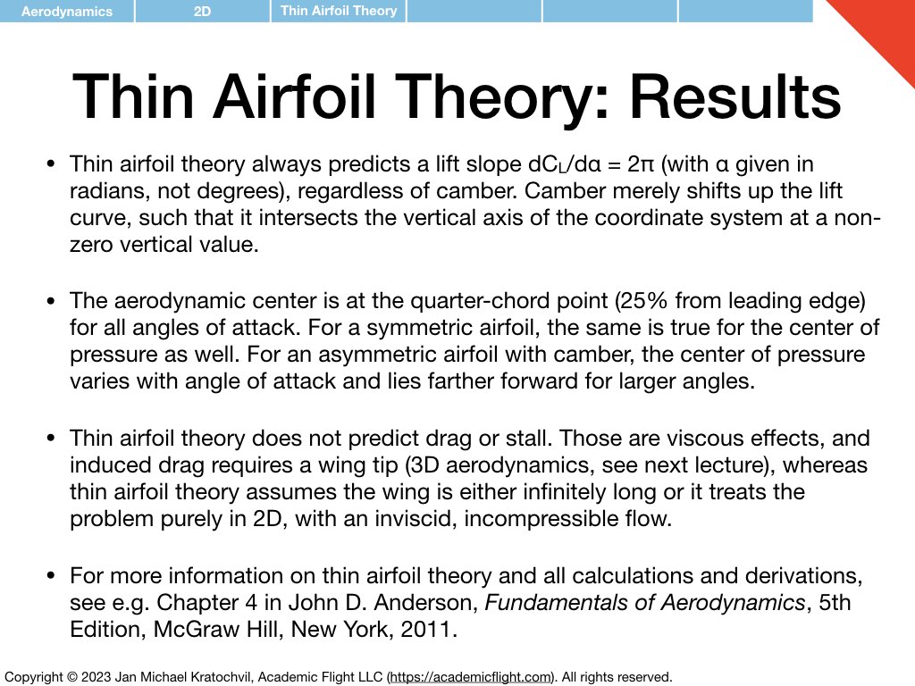
Some very fundamental aerodynamic concepts and theories common in aerospace engineering seem not to have made it into civilian pilot training. Those include the concept of circulation, which is related to lift in the Kutta-Joukowski theorem, the Kutta condition, the starting vortex, and thin airfoil theory. The slides below give brief summaries. Circulation is particularly important, because it forms the basis for Prandtl’s lifting line theory for a finite length wing, which becomes important, when we start discussing 3D aerodynamics seriously and will take a look at the wingtip vortices, which are not only responsible for the induced drag we have already encountered, but also pose a serious hazard to other aircraft in the wake of another.
Lift and Drag Equation Flowchart
For ambitious, advanced readers and participants in our online private pilot ground school, we provide a flowchart below, which shows the relations between various aerodynamic quantities related to lift and drag, as we have discussed in this lecture. The flowchart can be used to compute a variety of things, including reproducing most of the plots found in Chapters 4, 5, and 6 of the FAA Handbook of Aeronautical Knowledge (PHAK), such as the drag vs airspeed, D(V), plot or the increase of stall speed in a level turn as a function of load factor (or bank angle). That glide distance is independent of weight and that drag plays a negligible role in airspeed, while it is very important for glide distance, can also be easily inferred from this flowchart.
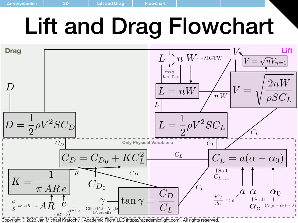
The reader is much encouraged to reproduce the plots in the PHAK themselves to improve their understanding and familiarity, for instance using Python and the Jupyter environment, which makes immediate plotting easy (they can be either installed for free with the Anaconda data science platform on one’s home computer or used over the internet with a free CoCalc account).