PPGS 2023-2024, Lecture 3: 3D Aerodynamics and Flight Dynamics – Selected Presentation Slides
3D Aerodynamics
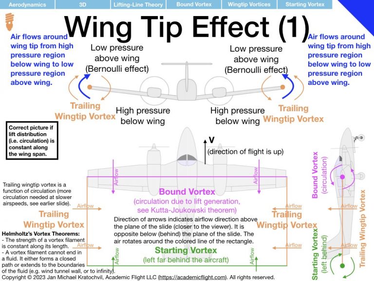
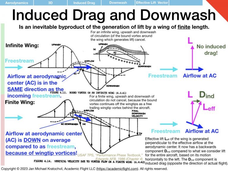
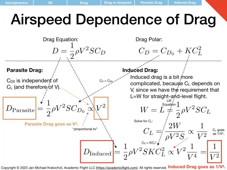
In the previous lecture we provided an introduction to basic 2D aerodynamics. We did encounter the phenomenon of induced drag, however, and noted that it is actually a 3D aerodynamic effect arising from the wing having finite length and the air flowing around the wingtips, from the high pressure region underneath the wing to the low pressure region above the wing.
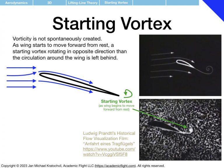
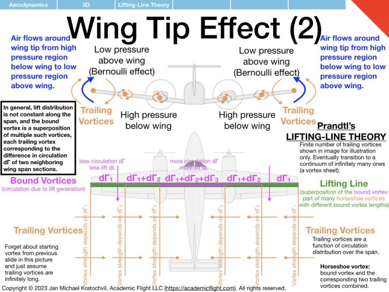
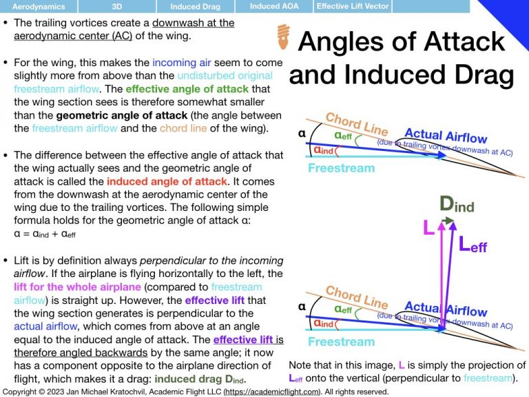
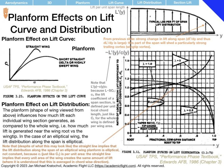
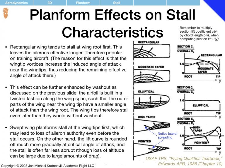
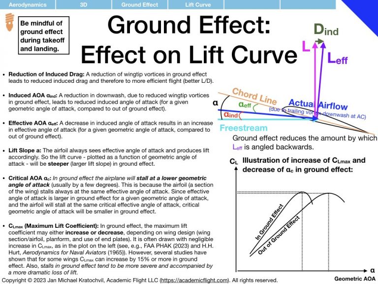
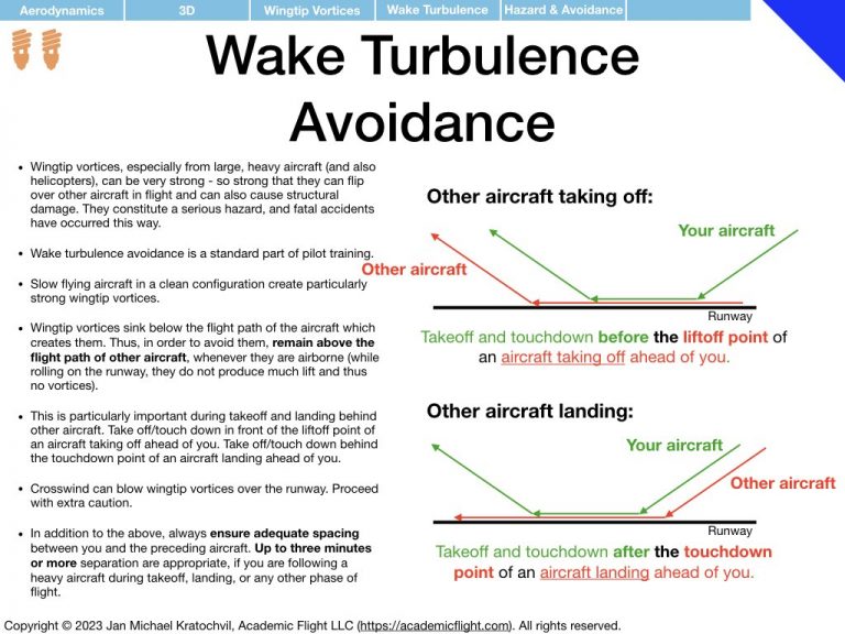
The resulting wingtip vortices from this airflow around the wingtips have profound effects, which are the topic of study in this lecture. They give rise to induced drag, alter the lift distribution along the wing span, cause an induced angle of attack which tilts the lift vector of wing sections backwards, and non-zero downwash is created not only at the aerodynamic center, but also far behind the wing. In addition, these wingtip vortices can also cause a serious hazard for other aircraft in flight (wake turbulence avoidance) and are attenuated near the ground, giving rise to more efficient flight in ground effect, within ca. 1/2-1 wing spans above the ground.
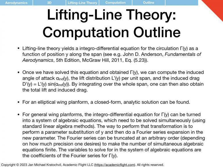
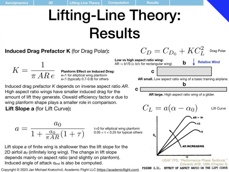
The presentation slides below explore some of these 3D aerodynamic concepts and their consequences, starting with a brief conceptual overview of Prandtl’s lifting-line theory.
The above is just a summary. Much more can and should be said about 3D aerodynamics, and the reader is highly encouraged to consult additional literature, such as:
- FAA handbooks (particularly the Pilot’s Handbook and Aeronautical Knowledge, 2023) and corresponding Advisory Circulars (e.g. AC 90-23G Aircraft Wake Turbulence), in particular in matters of safety. (As always, FAA materials take precedence in case of any discrepancies to any material presented on this website.)
- Hugh Harrison Hurt, Jr., Aerodynamics for Naval Aviators, NAVAIR 00-80T-80, Naval Air Systems Command, 1965 – for more details on theory and practical considerations for the advanced and performance-oriented pilot.
- John D. Anderson, Jr., Fundamentals of Aerodynamics, 5th Edition, McGraw Hill, 2011 – for a full mathematical treatment of Prandtl’s lifting-line theory in Section 5.3, including an analytical solution for the elliptical wing planform.
Flight Dynamics: Forces of Flight
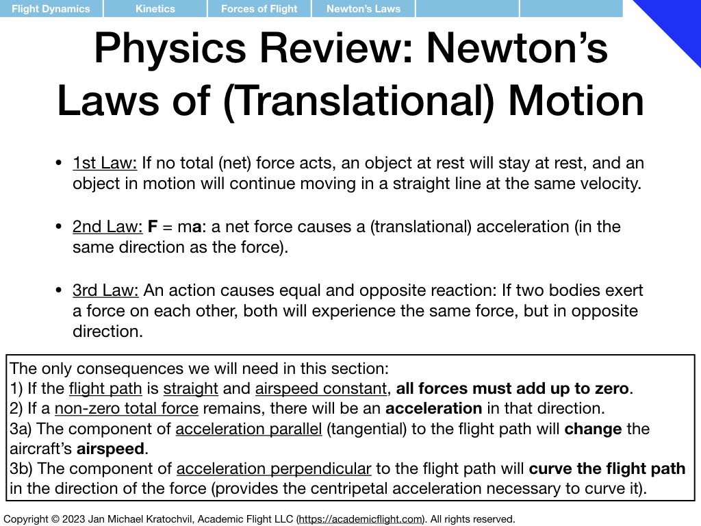
Until now we have concerned ourselves with how airflow causes aerodynamic forces. Now we shall turn to a different aspect of flight: assuming the forces are known, how do they affect the aircraft flight path and dynamics. Questions such as stall speed, glide distance, best glide speed, minimum sink speed, and load factor in a level turn all belong into this category, which we can answer by just considering forces and translational physics (rotational physics and moments will be discussed later; we shall not deal with aircraft attitude just yet).
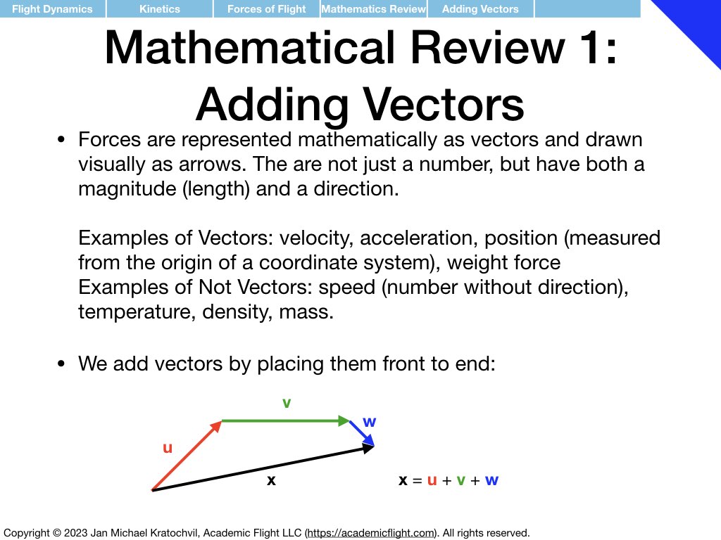
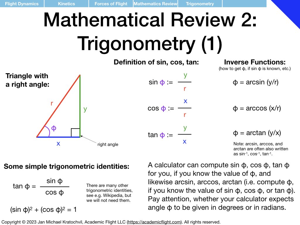
Math and Physics Review
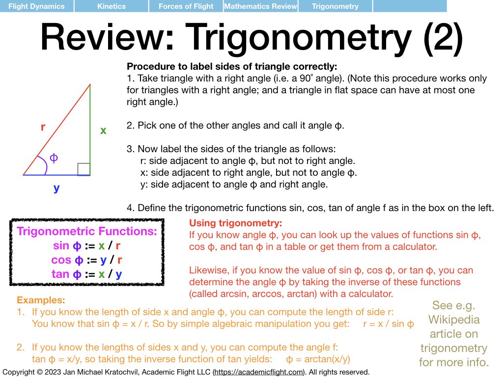
We offer a very brief review of Newton’s laws of motion, as well as how to add vectors and the very basics of trigonometry, to the extend we will be using them in this lecture.
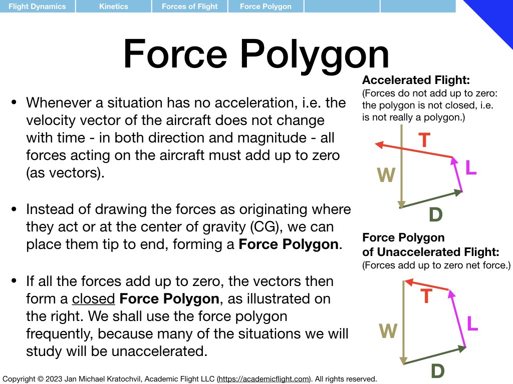
Fundamental Forces of Flight: General Procedure for Drawing the Forces of Flight
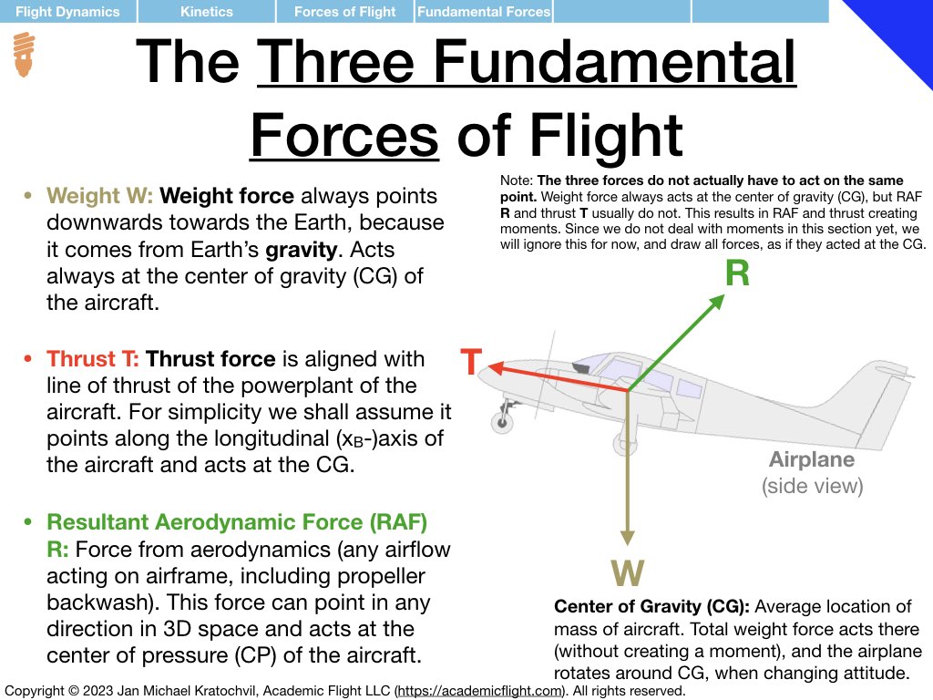
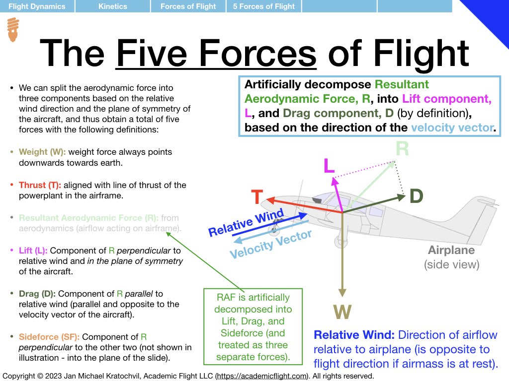
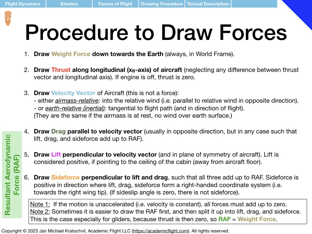
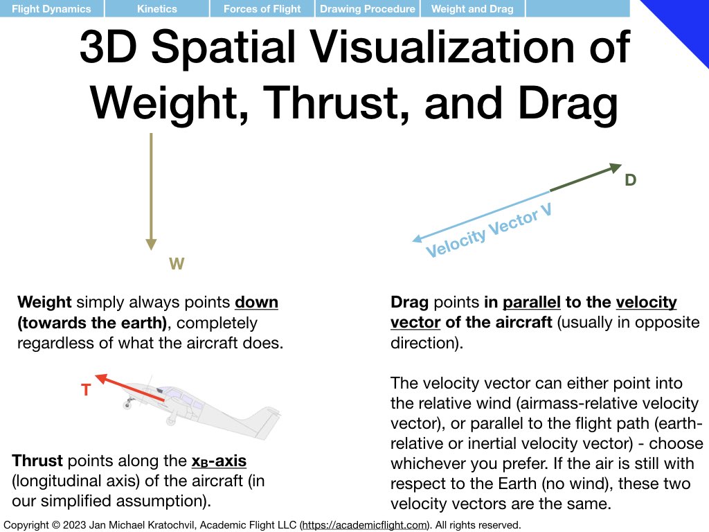
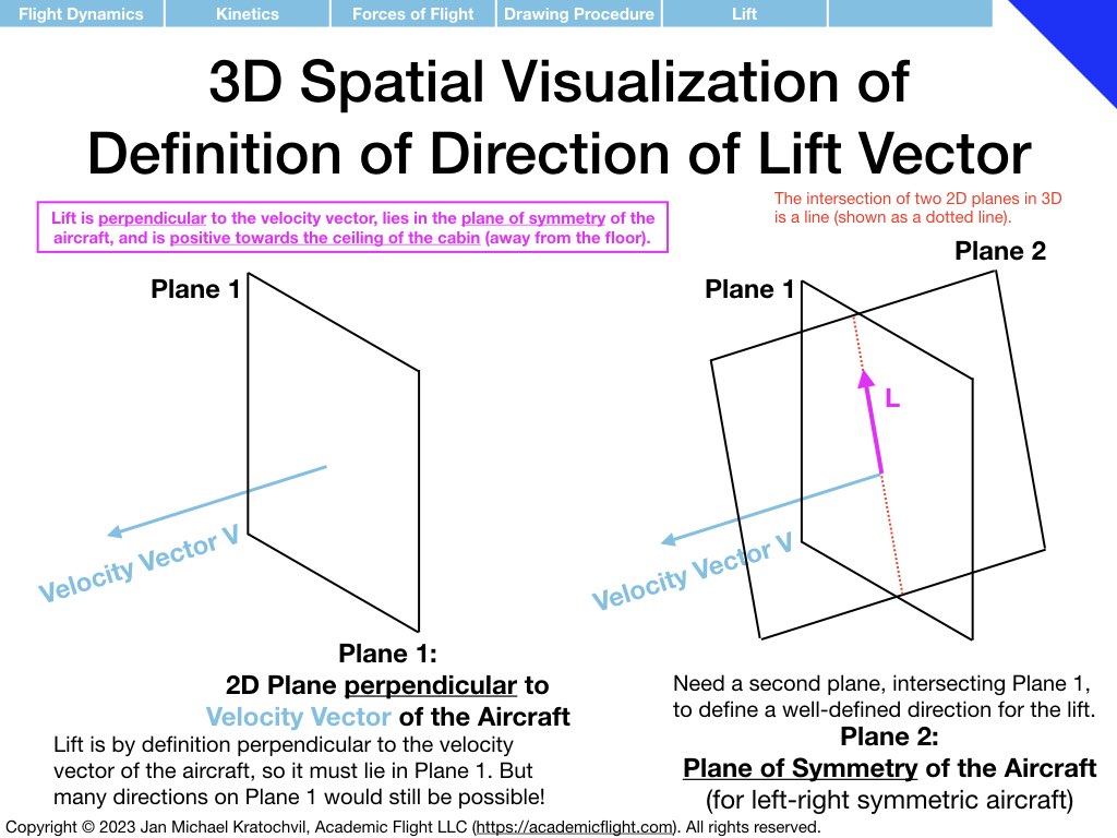
Our first step will be to identify the fundamental forces of flight, learn how to split them into their spatial components, and how to draw each one of them properly for any arbitrary flight situation. In our quest to do this properly, we discover that there are actually only three fundamental forces of flight, not four, as is commonly stated in most of flight training literature… Realizing that lift and drag are just two spatial components of one fundamental force, the resultant aerodynamic force (RAF), will help us greatly getting the force diagrams drawn correctly.
Application: Force Diagrams and Simple Conclusions for Specific Flight Situations
Now we are ready to apply the above drawing procedure for the forces of flight for weight, thrust, lift, drag, and sideforce to different situations in flight, which we routinely encounter as pilots. Our primary objective is to get some practice drawing the forces correctly and getting to know these flight situations a bit. But we also use this opportunity to draw some simple conclusions from our force diagrams right away.
From the presentation slides below, you will see that in this lecture, we managed to cover straight-and-level flight, climbing flight, and power-off gliding flight. Tutorial 3 covers additional situation, such as a glider climbing power-off in rising air, level turns, and spins.
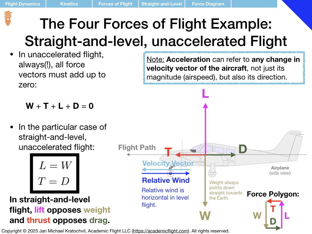
Steady, Straight-and-Level Flight
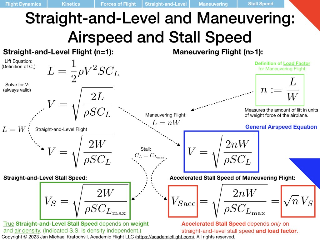
While discussing straight-and-level flight below, we also compute the (true) straight-and-level stall speed and notice its weight and air density dependence. We take this opportunity to compute the stall speed for maneuvering flight as well, by simply inserting the load factor \(n:=L/W\) into the calculation, and realize that the accelerated stall speed of maneuvering flight depends only on straight-and-level stall speed \(V_S\) and load factor \(n\). (In particular, as we shall appreciate next time, accelerated stall speed will not depend on bank angle in level turns directly, only via the load factor.)
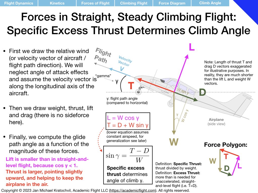
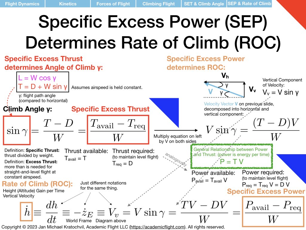
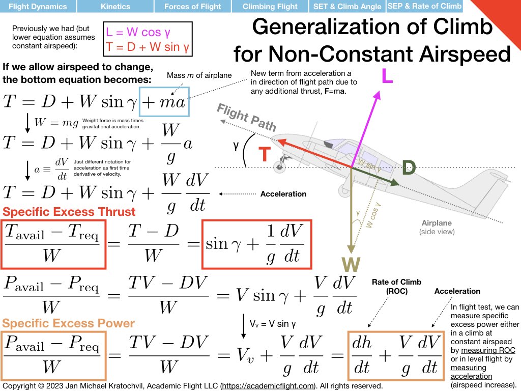
Steady, Climbing Flight (Power-On, in Still Air)
During our climbing flight discussion, we notice that specific excess thrust determines climb angle and specific excess power determines rate of climb (at constant airspeed). We also remark that in flight test, instead of using climb rate to measure specific excess power, we can also use acceleration in level flight instead, and we derive the corresponding equation for it (which method is preferable depends on the type of aircraft).
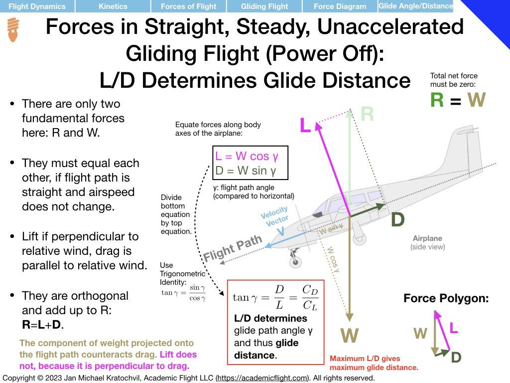
Gliding Flight (Power-Off, in Still Air)
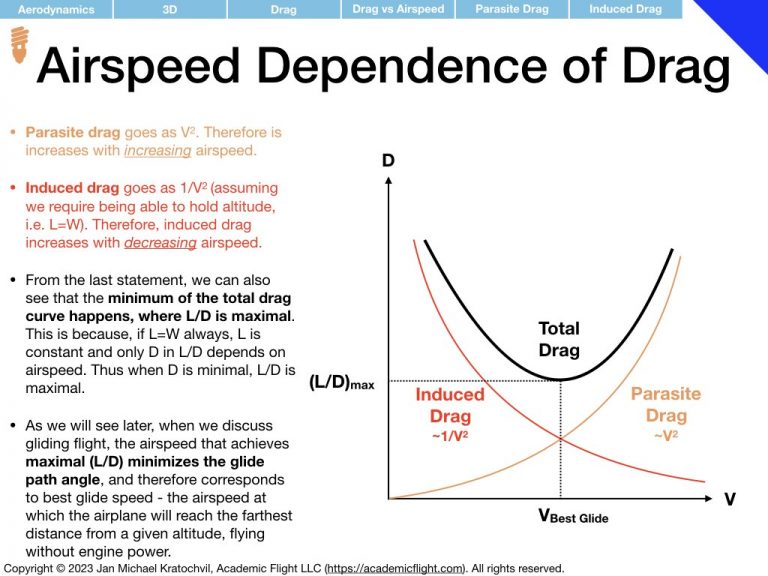
The slides below study straight, power-off gliding flight at constant airspeed in still air. First we draw the forces, then compare their lengths in the directions perpendicular to the velocity vector and parallel to the velcity vector of the aircraft to obtain the force equation(s) for gliding flight in components. (The slide says that this is done with respect to the airplane body axes – this is just a coincidence from the drawing, perpendicular and parallel to the velocity vector is really what is meant.) From these two equation we derive and equation for the glide path angle, which determines glide distance from a given altitude. Glide path angle depends strongly on lift and drag; in fact, it is related to the L/D ratio, with maximum L/D giving best glide distance. This is a very important result.
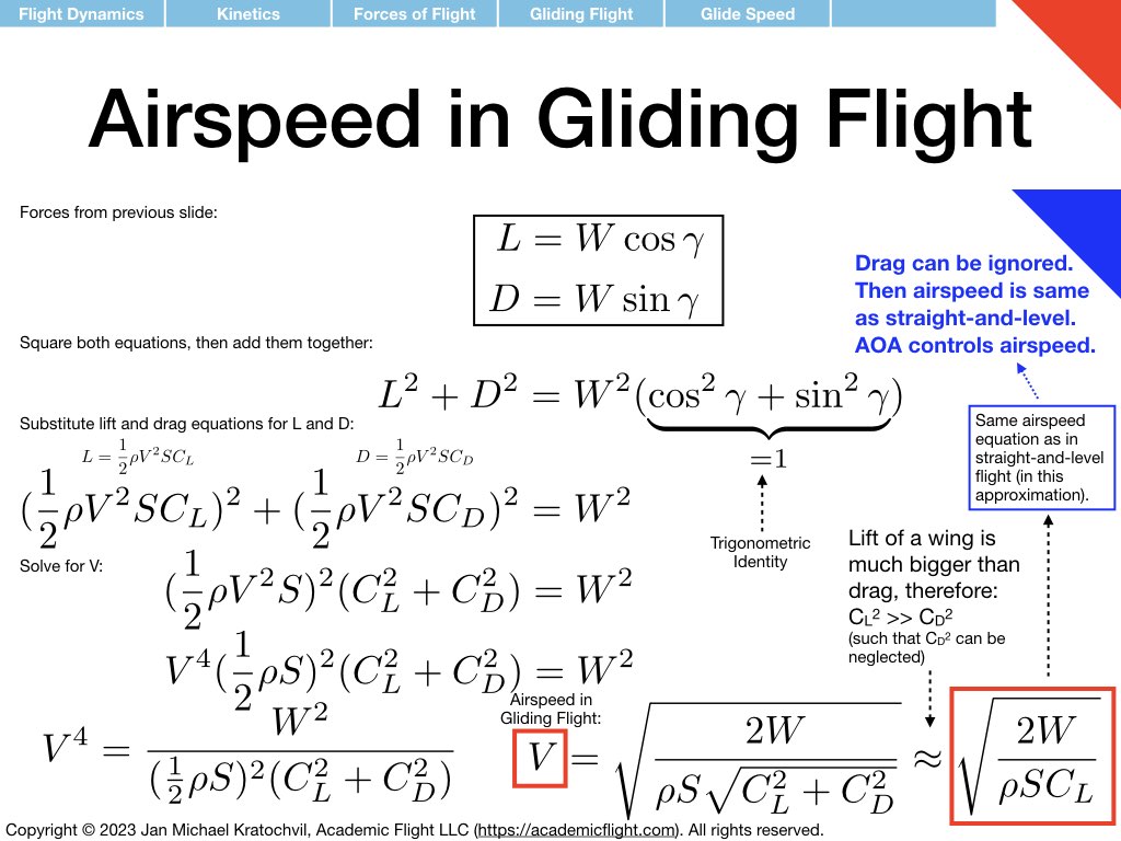
We then proceed to compute the airspeed in gliding flight, and find that in small glide path angle approximation the airspeed equation is (approximately) the same as in straight-and-level flight, and that drag has a negligible effect on airspeed.
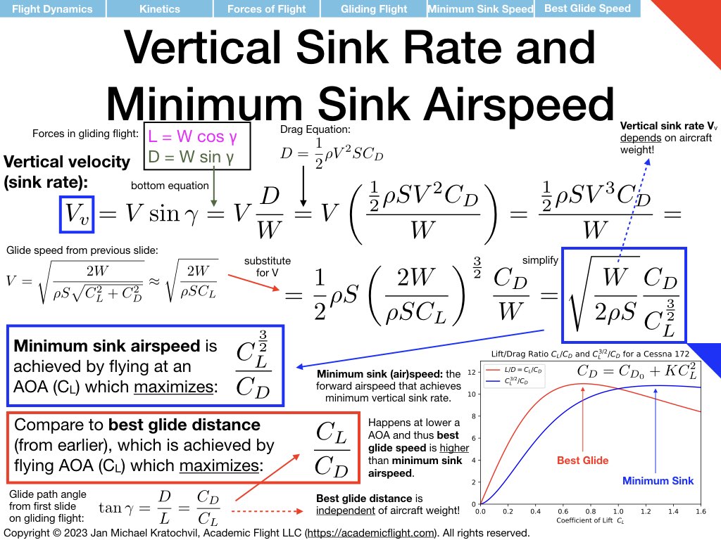
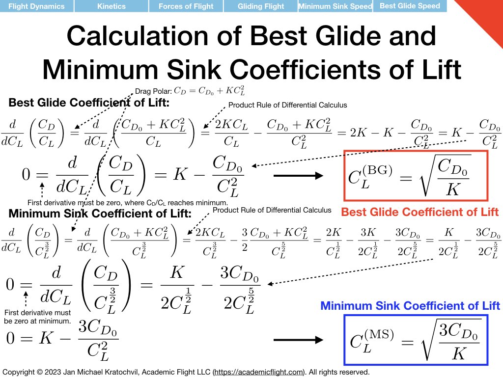
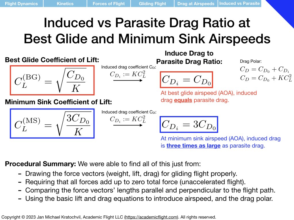
On the third slide we derive the formula for the vertical sink rate, and notice that minimum sink airspeed differs from best glide speed. On the fourth slide we compute the values of \(C_L\) for best glide and minimum sink, which turn out to depend only on the parameters \(C_{D_0}\) and \(K\) in the drag polar.
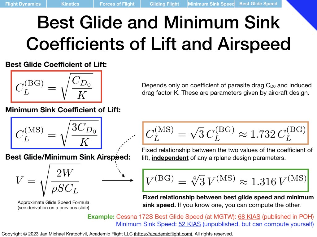
On the fifth slide, we notice that there is a fixed relationship between the values of \(C_L\) at best glide and minimum sink, and that their ratio is independent of any airplane parameters. The same thing is true for best glide and minimum sink speed: they differ by a constant factor independent of any airplane or environmental parameters, which is why, if one knows one, one can compute the other, which we do for the example of a Cessna 172S Skyhawk.
On the last slide, finally, we obtain the result that at best glide speed (best glide AOA), where L/D is maximal, induced drag \(C_{D_i}\) equals parasite drag \(C_{D_0}\). This is a statement we made earlier in the section on 3D Aerodynamics of this lecture already, but initially stated it without proof. We also derive that at minimum sink speed induced drag is three times as big as parasite drag.
Additional Flight Situations
The three situations above (straight-and-level flight, steady, straight climbs, and steady, straight, power-off glides) covered in the lecture are not enough for use to have sufficient practice with the force drawing procedure.
In Tutorial 3, which is associated with this lecture, you will be asked to use the above procedure to draw the forces in the additional fundamental flight situations listed below. In some of the problems, you will also be asked to write down the force equations parallel and perpendicular to the velocity vector, and to do some simple calculations in order to draw some conclusions. These situations are important for your understanding of flight and are an integral part of the lecture, so even if you do not actively try to do Tutorial 3, please do look at the Tutorial 3 Solution. The flight situations are:
- Power-off gliding flight (including computing glide distance and best glide and minimum sink speeds),
- Glider (without power) climbing in straight flight in a rising airmass (you will draw the lift and drag force vectors with respect to the airmass-relative or the earth-relative velocity vector).
- Level turn (you will also be asked to compute the relationship between load factor and bank angle, which will allow you to determine accelerated stall speed in a level turn based on bank angle),
- Spin (you will start with drawing the forces in a prototype spin falling straight down, and then generalize it to helical flight path along the spin axis).
Note that power-off gliding flight was originally treated in the tutorial, so we left it in there, but a more thorough treatment of gliding flight has been since incorporated into the main body of this lecture above already (so this is a bit of a duplication in the tutorial – consider it a warm up problem, you should already know how to solve from the lecture).